Computing Centralities

cityseer is a Python package for computing network centralities on street networks. It handles network cleaning, coordinate-aware shortest paths, and scales to tens of thousands of edges. You’ll use it here to compute closeness and betweenness centralities for Madrid’s street network.

# uncomment to install cityseer
# !pip install cityseer

Ignore!

This block just silences the output from cityseer, which makes for neater notebook outputs, but you probably don’t want to do this in Colab where the progress bars would be useful.

import os
os.environ["CITYSEER_QUIET_MODE"] = '1'

Download the Street Network and Modified Street Network for Madrid. Use geopandas to open them. Update the file path as necessary.

import geopandas as gpd
import matplotlib.pyplot as plt
from cityseer.metrics import networks
from cityseer.tools import graphs, io

# update the file path as needed
mad_net = gpd.read_file("../../data/madrid_streets/street_network_mod.gpkg")

mad_net.head()

	clased	nombre	geometry
0	Autopista libre / autovía	M-406	LINESTRING (437440 4460857, 437460 4460868, 43...
1	Carretera convencional	M-406	LINESTRING (437438 4460861, 437472 4460878)
2	Urbano	FUERZAS ARMADAS (DE LAS)	LINESTRING (438131 4461473, 438133 4461461, 43...
3	Urbano	FUERZAS ARMADAS (DE LAS)	LINESTRING (438023 4461398, 438058 4461407, 43...
4	Carretera convencional	M-406	LINESTRING (438181 4461468, 438177 4461465, 43...

Use the cityseer io module’s nx_from_generic_geopandas() method to convert the GeoDataFrame to a networkX graph.

# cityseer expects single-part geometries
# explode splits any MultiLineStrings into individual LineStrings
mad_net = mad_net.explode().reset_index(drop=True)

# convert from geopandas to networkX
mad_net_nx = io.nx_from_generic_geopandas(mad_net)

# print number of nodes and edges
mad_net_nx.number_of_nodes(), mad_net_nx.number_of_edges()

WARNING:cityseer.tools.io:Dropping zero length edge at row index 49094
INFO:cityseer.tools.graphs:Merging parallel edges within buffer of 1.

(56260, 83295)

cityseer builds a networkX graph from the GeoDataFrame. In this primal representation, nodes represent street intersections (with x and y coordinates) and edges represent street segments (with their full geometry). This means shortest-path algorithms can now calculate street lengths and angular deviation over the network.

The dual representation swaps this: each street segment becomes a node, and connections between segments become edges. Centralities computed on the dual graph describe street segments directly, which makes them easier to visualise and interpret. Convert with the nx_to_dual method.

# convert the network to its dual representation
mad_net_dual_nx = graphs.nx_to_dual(mad_net_nx)

# print number of nodes and edges
mad_net_dual_nx.number_of_nodes(), mad_net_dual_nx.number_of_edges()

INFO:cityseer.tools.graphs:Converting graph to dual.
INFO:cityseer.tools.graphs:Preparing dual nodes
INFO:cityseer.tools.graphs:Preparing dual edges (splitting and welding geoms)

(83295, 178022)

Each node in a cityseer network has a live attribute. When live is True, centralities are computed for that node. When False, the node is still included in shortest-path calculations (as buffer) but receives no centrality value. This is how localised analysis avoids edge effects: include the surrounding network for routing, but only report results for the area of interest.

Load a boundary for central Madrid and set live=True for nodes that fall inside it. The Point constructor and contains() method from shapely handle the spatial test.

from shapely.geometry import Point

# load the boundary
boundary_gdf = gpd.read_file("../../data/bounds_small.gpkg")
boundary_geom = boundary_gdf.union_all()

# set live=True for nodes inside the boundary
for node, data in mad_net_dual_nx.nodes(data=True):
    pt = Point(data["x"], data["y"])
    data["live"] = boundary_geom.contains(pt)

# count live vs buffer nodes
n_live = sum(1 for _, d in mad_net_dual_nx.nodes(data=True) if d.get("live"))
n_total = mad_net_dual_nx.number_of_nodes()
print(f"Live: {n_live}, Buffer: {n_total - n_live}, Total: {n_total}")

Live: 13702, Buffer: 69593, Total: 83295

Next, create a NetworkStructure using the cityseer io module’s network_structure_from_nx() method. The method returns three items:

nodes_gdf: A geopandas dataframe with the nodes of the network. Since we are working with a dual representation, these are the midpoints of the original street segments (but are visualised as the street segments themselves);
edges_gdf: A geopandas dataframe with the linkages from segment to segment (metric and geometric distances are calculated from these);
network_structure: A cityseer NetworkStructure object which is used for optimised network analysis.

# create a network structure
nodes_gdf, edges_gdf, network_structure = io.network_structure_from_nx(mad_net_dual_nx)

nodes_gdf.head()

INFO:cityseer.tools.io:Preparing node and edge arrays from networkX graph.
INFO:cityseer.graph:Edge R-tree built successfully with 178022 items.

	ns_node_idx	x	y	live	weight	primal_edge	primal_edge_node_a	primal_edge_node_b	dual_node
x437440.0-y4460857.0_x437472.0-y4460878.0_k0	0	437456.843465	4.460866e+06	False	1	LINESTRING (437440 4460857, 437460 4460868, 43...	x437440.0-y4460857.0	x437472.0-y4460878.0	POINT (437456.843465 4460866.263906)
x437399.0-y4460843.0_x437440.0-y4460857.0_k0	1	437419.500000	4.460850e+06	False	1	LINESTRING (437399 4460843, 437440 4460857)	x437440.0-y4460857.0	x437399.0-y4460843.0	POINT (437419.5 4460850)
x437438.0-y4460861.0_x437472.0-y4460878.0_k0	2	437455.000000	4.460870e+06	False	1	LINESTRING (437438 4460861, 437472 4460878)	x437472.0-y4460878.0	x437438.0-y4460861.0	POINT (437455 4460869.5)
x437472.0-y4460878.0_x438164.0-y4461448.0_k0	3	437789.634847	4.461205e+06	False	1	LINESTRING (437472 4460878, 437488 4460890, 43...	x437472.0-y4460878.0	x438164.0-y4461448.0	POINT (437789.634847 4461204.897709)
x437399.0-y4460848.0_x437438.0-y4460861.0_k0	4	437418.500000	4.460854e+06	False	1	LINESTRING (437399 4460848, 437438 4460861)	x437438.0-y4460861.0	x437399.0-y4460848.0	POINT (437418.5 4460854.5)

Plot the dual segments to see what we’re working with.

# plot the dual network
ax = nodes_gdf.plot(linewidth=1, color="red", figsize=(8, 8))

ax.set_xlim(438000, 438000 + 6000)
ax.set_ylim(4472000, 4472000 + 6000)
ax.axis(False)

(np.float64(438000.0),
 np.float64(444000.0),
 np.float64(4472000.0),
 np.float64(4478000.0))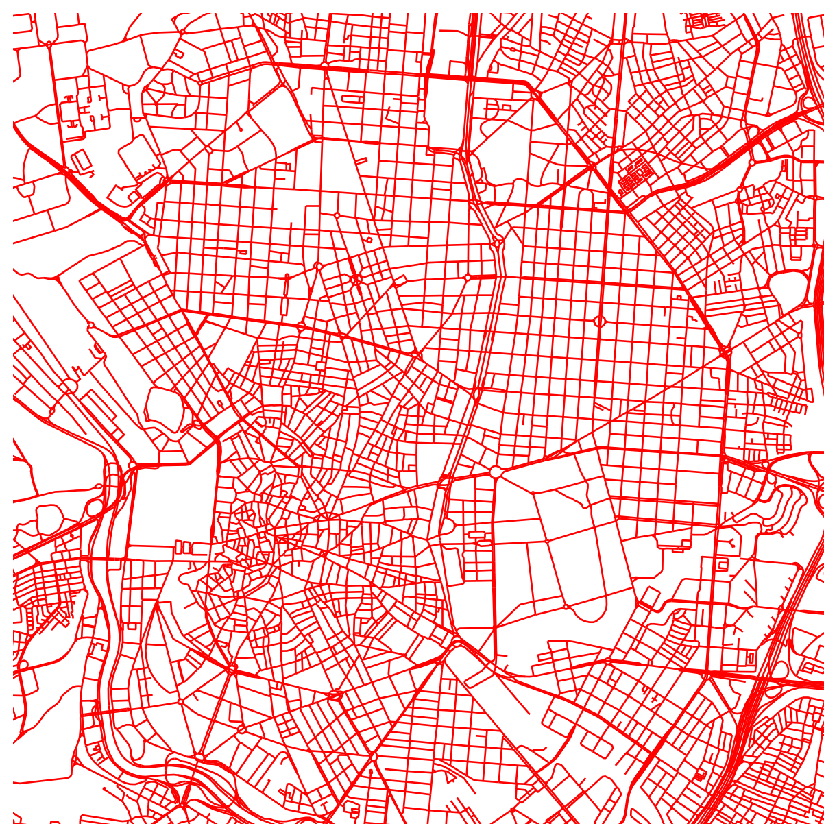

Start with metric distance centralities using the node_centrality_shortest() method from the cityseer networks module.

This requires three core arguments:

A NetworkStructure object;
The nodes_gdf GeoDataFrame which will be used to store the results;
A list of distance thresholds for which to compute the centralities.

# compute shortest path node centralities
nodes_gdf = networks.node_centrality_shortest(
    # the network structure on which to compute the measures
    network_structure=network_structure,
    # the nodes GeoDataFrame to which the results will be written
    nodes_gdf=nodes_gdf,
    # the distance thresholds for computing centralities - set this as wanted
    distances=[400, 800],
)

# the results are now in the nodes GeoDataFrame
nodes_gdf.head()

INFO:cityseer.metrics.networks:Computing node centrality (shortest).
INFO:cityseer.metrics.networks:  Full: 400m, 800m

	ns_node_idx	x	y	live	weight	primal_edge	primal_edge_node_a	primal_edge_node_b	dual_node	...	cc_hillier_400	cc_hillier_800
x437440.0-y4460857.0_x437472.0-y4460878.0_k0	0	437456.843465	4.460866e+06	False	1	LINESTRING (437440 4460857, 437460 4460868, 43...	x437440.0-y4460857.0	x437472.0-y4460878.0	POINT (437456.843465 4460866.263906)	...	NaN	NaN
x437399.0-y4460843.0_x437440.0-y4460857.0_k0	1	437419.500000	4.460850e+06	False	1	LINESTRING (437399 4460843, 437440 4460857)	x437440.0-y4460857.0	x437399.0-y4460843.0	POINT (437419.5 4460850)	...	NaN	NaN
x437438.0-y4460861.0_x437472.0-y4460878.0_k0	2	437455.000000	4.460870e+06	False	1	LINESTRING (437438 4460861, 437472 4460878)	x437472.0-y4460878.0	x437438.0-y4460861.0	POINT (437455 4460869.5)	...	NaN	NaN
x437472.0-y4460878.0_x438164.0-y4461448.0_k0	3	437789.634847	4.461205e+06	False	1	LINESTRING (437472 4460878, 437488 4460890, 43...	x437472.0-y4460878.0	x438164.0-y4461448.0	POINT (437789.634847 4461204.897709)	...	NaN	NaN
x437399.0-y4460848.0_x437438.0-y4460861.0_k0	4	437418.500000	4.460854e+06	False	1	LINESTRING (437399 4460848, 437438 4460861)	x437438.0-y4460861.0	x437399.0-y4460848.0	POINT (437418.5 4460854.5)	...	NaN	NaN

5 rows × 26 columns

The results are stored in the nodes_gdf GeoDataFrame, where you’ll note the addition of a number of columns prefixed with cc_ for different forms of centrality. The numbers represent the distance threshold at which the centrality was computed.

nodes_gdf.columns

Index(['ns_node_idx', 'x', 'y', 'live', 'weight', 'primal_edge',
       'primal_edge_node_a', 'primal_edge_node_b', 'primal_edge_idx',
       'dual_node', 'cc_beta_400', 'cc_beta_800', 'cc_cycles_400',
       'cc_cycles_800', 'cc_density_400', 'cc_density_800', 'cc_farness_400',
       'cc_farness_800', 'cc_harmonic_400', 'cc_harmonic_800',
       'cc_hillier_400', 'cc_hillier_800', 'cc_betweenness_400',
       'cc_betweenness_800', 'cc_betweenness_beta_400',
       'cc_betweenness_beta_800'],
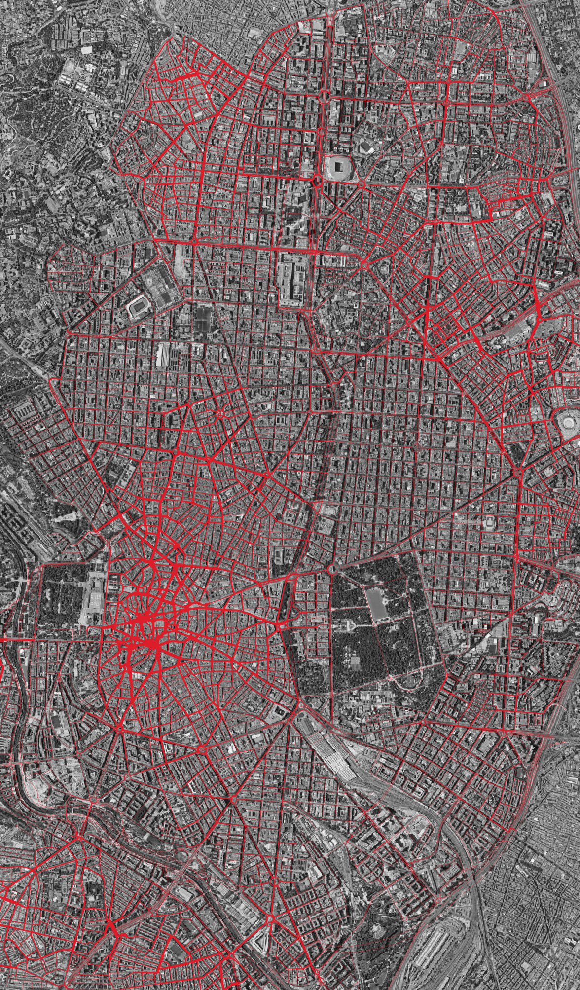
      dtype='str')

Use the built-in GeoDataFrame plot functionality to visualise harmonic closeness centrality at a 400m distance.

# this sets up the figure and axis as wanted
fig, ax = plt.subplots(figsize=(8, 8))
fig.set_facecolor("#111")

# this plots the values for the selected column
nodes_gdf.plot(
    column="cc_harmonic_400",
    cmap="magma",
    linewidth=1,
    ax=ax,
)

# set the axis limits
ax.set_xlim(438000, 438000 + 6000)
ax.set_ylim(4472000, 4472000 + 6000)
# turn off the axis
ax.axis(False)

(np.float64(438000.0),
 np.float64(444000.0),
 np.float64(4472000.0),
 np.float64(4478000.0))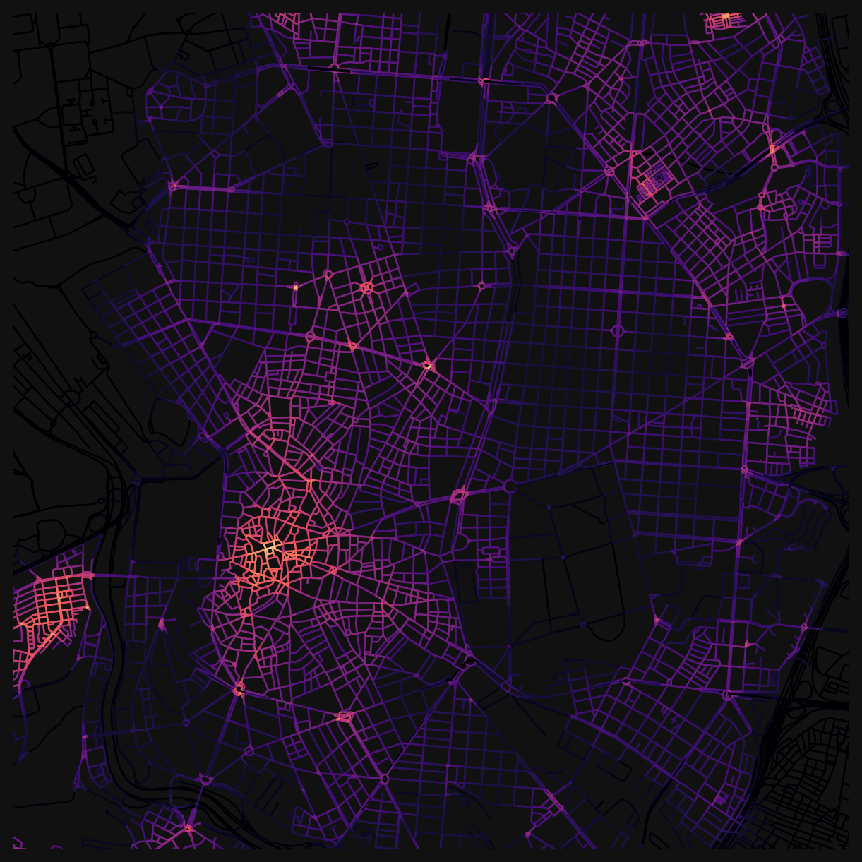

The same pattern can be used for geometric distance (angular or ‘simplest-path’) centralities by using the node_centrality_simplest() method.

# simplest path node centralities are computed similarly
nodes_gdf = networks.node_centrality_simplest(
    network_structure=network_structure,
    nodes_gdf=nodes_gdf,
    distances=[400, 800],
)

nodes_gdf.head()

INFO:cityseer.metrics.networks:Computing node centrality (simplest).
INFO:cityseer.metrics.networks:  Full: 400m, 800m

	ns_node_idx	x	y	live	weight	primal_edge	primal_edge_node_a	primal_edge_node_b	dual_node	...	cc_hillier_400_ang	cc_hillier_800_ang
x437440.0-y4460857.0_x437472.0-y4460878.0_k0	0	437456.843465	4.460866e+06	False	1	LINESTRING (437440 4460857, 437460 4460868, 43...	x437440.0-y4460857.0	x437472.0-y4460878.0	POINT (437456.843465 4460866.263906)	...	NaN	NaN
x437399.0-y4460843.0_x437440.0-y4460857.0_k0	1	437419.500000	4.460850e+06	False	1	LINESTRING (437399 4460843, 437440 4460857)	x437440.0-y4460857.0	x437399.0-y4460843.0	POINT (437419.5 4460850)	...	NaN	NaN
x437438.0-y4460861.0_x437472.0-y4460878.0_k0	2	437455.000000	4.460870e+06	False	1	LINESTRING (437438 4460861, 437472 4460878)	x437472.0-y4460878.0	x437438.0-y4460861.0	POINT (437455 4460869.5)	...	NaN	NaN
x437472.0-y4460878.0_x438164.0-y4461448.0_k0	3	437789.634847	4.461205e+06	False	1	LINESTRING (437472 4460878, 437488 4460890, 43...	x437472.0-y4460878.0	x438164.0-y4461448.0	POINT (437789.634847 4461204.897709)	...	NaN	NaN
x437399.0-y4460848.0_x437438.0-y4460861.0_k0	4	437418.500000	4.460854e+06	False	1	LINESTRING (437399 4460848, 437438 4460861)	x437438.0-y4460861.0	x437399.0-y4460848.0	POINT (437418.5 4460854.5)	...	NaN	NaN

5 rows × 38 columns

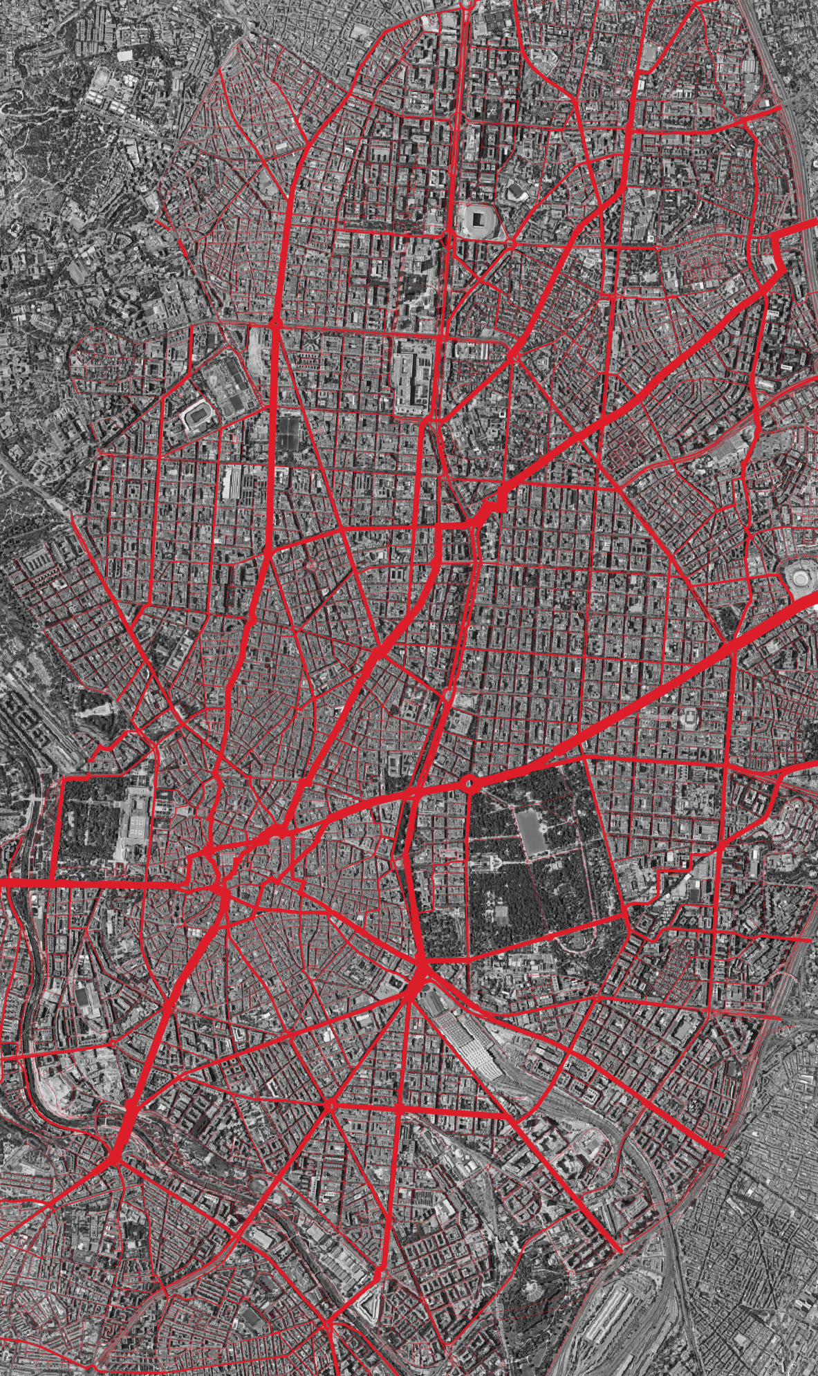
Angular centrality columns are suffixed with ang. Plot angular harmonic closeness centrality at 800m.

fig, ax = plt.subplots(figsize=(8, 8))
fig.set_facecolor("#111")

nodes_gdf.plot(
    column="cc_harmonic_800_ang",
    cmap="magma",
    linewidth=1,
    ax=ax,
)

ax.set_xlim(438000, 438000 + 6000)
ax.set_ylim(4472000, 4472000 + 6000)
ax.axis(False)

(np.float64(438000.0),
 np.float64(444000.0),
 np.float64(4472000.0),
 np.float64(4478000.0))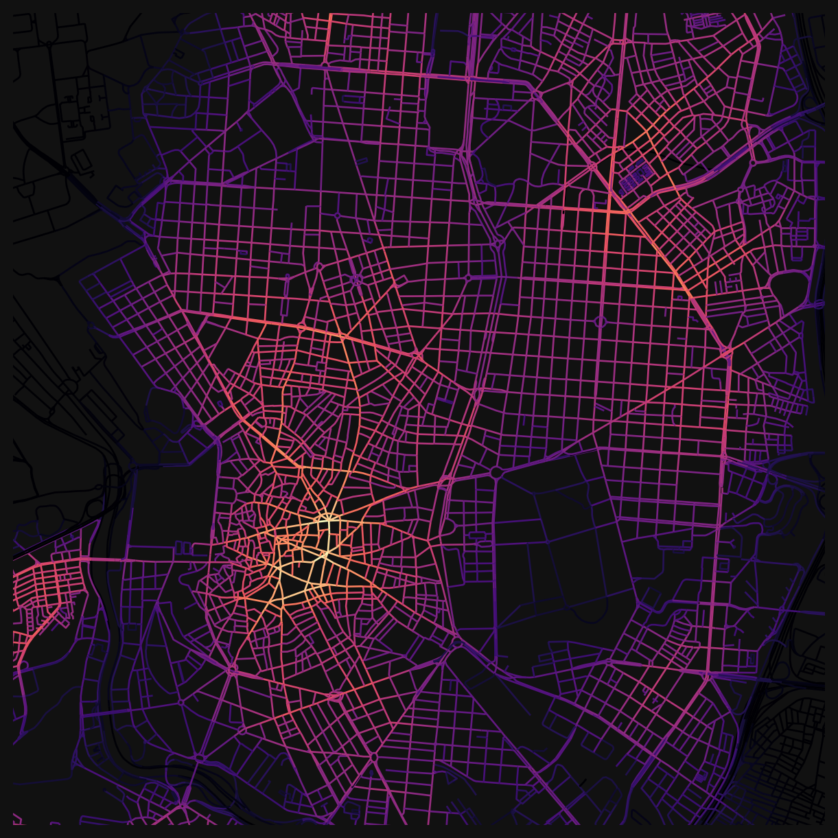

Different distance thresholds reveal different structures. The images at the top of this page show the contrast: at 800m, betweenness picks out local through-routes within neighbourhoods, while at 10km, the city-wide arterials dominate.

Tip

You can use this workflow to compare scenarios: prepare two networks (e.g. before and after a road closure), compute centralities for each, save the results with to_file(), and compare them in QGIS or Python.

Saving data

The data can be saved to an output .gpkg, which can be used in QGIS for visualisation and analysis.

# uncomment to save the nodes dataframe to a file for use from QGIS
# nodes_gdf.to_file('centralities.gpkg')

Challenges

Compute additional distances

Using the same patterns as before, compute centralities for the following additional distances: 1200m, 1600m, and 2000m (you can also try larger distances like 5km or 10km). Once complete, plot the angular betweenness centrality for 2000m.

Interventions at Paseo del Prado

Modify Madrid’s street network, recompute centralities, and evaluate the impact of your changes.

Inspect the street_network for Madrid, focusing on the region around Paseo del Prado.

Can you spot missing linkages in your network? e.g. pedestrian crossings that exist in reality but are missing from the network file.
What changes would you make to the network to improve East/West pedestrian connectivity and access to the park from the city centre?

Compute the centralities for the changed network. Then visually compare the centralities of the original network with the centralities of the changed network in QGIS. What differences do you observe?

Tip

When comparing centralities across networks, use the same colour scale and style settings for both plots to ensure that the differences are visually comparable.

References

Solutions

Compute additional distances

Solution

nodes_gdf = networks.node_centrality_shortest(
    network_structure=network_structure,
    nodes_gdf=nodes_gdf,
    distances=[1200, 1600, 2000],
)
nodes_gdf = networks.node_centrality_simplest(
    network_structure=network_structure,
    nodes_gdf=nodes_gdf,
    distances=[1200, 1600, 2000],
)

fig, ax = plt.subplots(figsize=(8, 8))
fig.set_facecolor("#111")

nodes_gdf.plot(
    column="cc_betweenness_2000_ang",
    cmap="magma",
    linewidth=1,
    ax=ax,
)

ax.set_xlim(438000, 438000 + 6000)
ax.set_ylim(4472000, 4472000 + 6000)
ax.axis(False)

INFO:cityseer.metrics.networks:Computing node centrality (shortest).
INFO:cityseer.metrics.networks:  Full: 1200m, 1600m, 2000m
INFO:cityseer.metrics.networks:Computing node centrality (simplest).
INFO:cityseer.metrics.networks:  Full: 1200m, 1600m, 2000m

(np.float64(438000.0),
 np.float64(444000.0),
 np.float64(4472000.0),
 np.float64(4478000.0))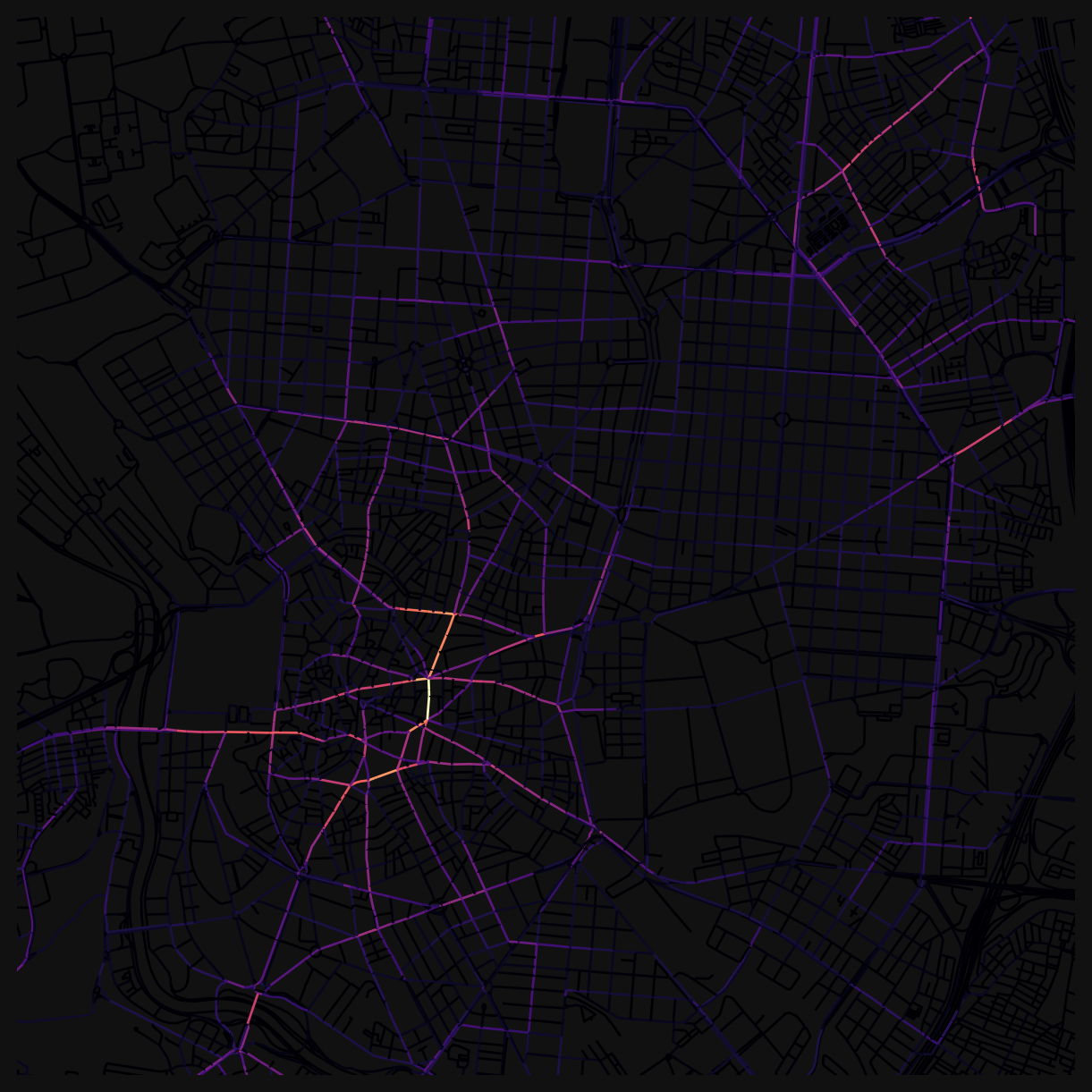

Bonus

The before and after intervention scenarios can be compared visually in QGIS, where you manually query features to see what the relative impact on the centrality values is. Here is a more advanced example using Python and the GeoPandas package to automate this.

The two networks (original and modified) have different street segments, so you cannot directly compare centrality values by feature ID. Instead, you need a spatial approach to match segments across datasets and compute the difference.

This example:

Prepares both the original and modified centrality results.
Performs a spatial join to pair each segment in the modified network with its nearest counterpart in the original network.
Computes the difference in a centrality metric (e.g. angular betweenness at 2000m) between matched segments.
Plots the result so you can see which streets gained or lost centrality.

Load and process the original (unmodified) network through the same pipeline.

# load the original network
orig_net = gpd.read_file("../../data/madrid_streets/street_network.gpkg")
orig_net = orig_net.explode().reset_index(drop=True)

# convert to networkX and dual representation
orig_nx = io.nx_from_generic_geopandas(orig_net)
orig_dual_nx = graphs.nx_to_dual(orig_nx)

# set live nodes using the same boundary
for node, data in orig_dual_nx.nodes(data=True):
    pt = Point(data["x"], data["y"])
    data["live"] = boundary_geom.contains(pt)

# build network structure
orig_nodes_gdf, orig_edges_gdf, orig_network_structure = io.network_structure_from_nx(orig_dual_nx)

# compute centralities at the same distances
orig_nodes_gdf = networks.node_centrality_simplest(
    network_structure=orig_network_structure,
    nodes_gdf=orig_nodes_gdf,
    distances=[2000],
)

# compute 2000m simplest-path centrality for the modified network too
nodes_gdf = networks.node_centrality_simplest(
    network_structure=network_structure,
    nodes_gdf=nodes_gdf,
    distances=[2000],
)

INFO:cityseer.tools.graphs:Merging parallel edges within buffer of 1.
INFO:cityseer.tools.graphs:Converting graph to dual.
INFO:cityseer.tools.graphs:Preparing dual nodes
INFO:cityseer.tools.graphs:Preparing dual edges (splitting and welding geoms)
INFO:cityseer.tools.io:Preparing node and edge arrays from networkX graph.
INFO:cityseer.graph:Edge R-tree built successfully with 177955 items.
INFO:cityseer.metrics.networks:Computing node centrality (simplest).
INFO:cityseer.metrics.networks:  Full: 2000m
INFO:cityseer.metrics.networks:Computing node centrality (simplest).
INFO:cityseer.metrics.networks:  Full: 2000m

The two networks have different edges, so feature IDs won’t match. Use a spatial join to pair each segment in the modified network with its nearest counterpart in the original. A max_distance threshold (here 50m) avoids pairing segments that have no real match: new or deleted edges get NaN instead of being matched to something far away.

# the dual network's geometry column is the primal edge (linestrings)
# create point-based GeoDataFrames for the spatial join using the node x/y
mod_pts = gpd.GeoDataFrame(
    {
        "betw_mod": nodes_gdf["cc_betweenness_2000_ang"].values,
        "primal_edge": nodes_gdf["primal_edge"].values,
    },
    geometry=gpd.points_from_xy(nodes_gdf["x"], nodes_gdf["y"]),
    crs=nodes_gdf.crs,
)
orig_pts = gpd.GeoDataFrame(
    {"betw_orig": orig_nodes_gdf["cc_betweenness_2000_ang"].values},
    geometry=gpd.points_from_xy(orig_nodes_gdf["x"], orig_nodes_gdf["y"]),
    crs=orig_nodes_gdf.crs,
)

# pair each modified segment with the nearest original segment
joined = gpd.sjoin_nearest(
    mod_pts,
    orig_pts,
    how="left",
    max_distance=50,
)

# drop duplicate matches and compute the difference
joined = joined[~joined.index.duplicated(keep="first")]
joined["delta_betw_2000_ang"] = joined["betw_mod"] - joined["betw_orig"]

# restore line geometry for plotting
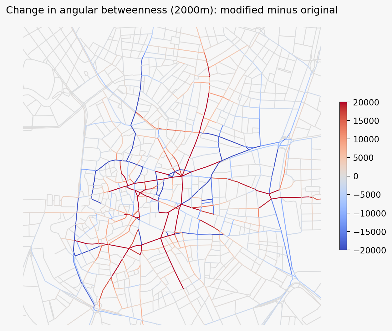
joined = joined.set_geometry("primal_edge")

Plot the difference. Positive values indicate segments that gained angular betweenness in the modified network; negative values indicate segments that lost it.

# save the result to a file for use in QGIS
# drop the point geometry column left over from the spatial join
# joined.drop(columns=["geometry"]).to_file("centrality_diff.gpkg")

fig, ax = plt.subplots(figsize=(8, 8))
fig.set_facecolor("#f7f7f7")

joined.plot(
    column="delta_betw_2000_ang",
    cmap="coolwarm",
    vmin=-20000,
    vmax=20000,
    linewidth=1,
    legend=True,
    legend_kwds={"shrink": 0.4},
    ax=ax,
)

ax.set_xlim(439000, 439500 + 2000)
ax.set_ylim(4473000, 4473500 + 2000)
ax.axis(False)
ax.set_title("Change in angular betweenness (2000m): modified minus original")

Text(0.5, 1.0, 'Change in angular betweenness (2000m): modified minus original')