Thermal Comfort in Bilbao
Datasets
Download the following from the datasets page:
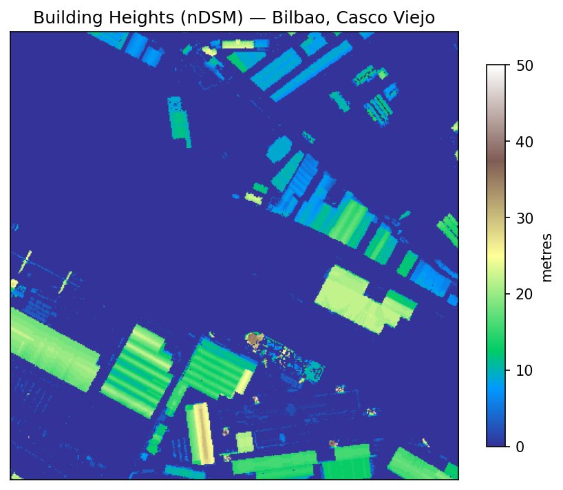
- BDSM.tif - Normalised Digital Surface Model. Building heights above ground level, derived from LiDAR. 2.5m resolution.
- CDSM.tif - Canopy Digital Surface Model. Vegetation heights above ground. 2.5m resolution.
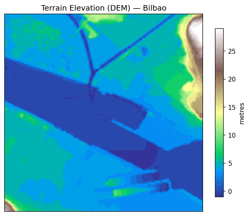
- DEM.tif - Digital Elevation Model. Terrain baseline. 5m resolution.
The rasters cover a 3.4km x 3.4km area of Bilbao in EPSG:25830 (ETRS89 / UTM zone 30N). In Step 3, you’ll set a 1km x 1km processing extent so the plugin only computes within that area.
Install the SOLWEIG plugin
The SOLWEIG plugin requires QGIS 4.0 or a recent nightly build (3.99+). It will not appear in the Plugin Manager on QGIS 3.x.
- Open QGIS and go to
Plugins>Manage and Install Plugins. - In the Settings tab, enable
Show also experimental plugins. - Search for SOLWEIG and install it.
- On first use, the plugin will prompt you to install the
solweigPython library. Accept the prompt and wait for installation to complete. - Once installed, you’ll find three SOLWEIG algorithms in the Processing Toolbox under SOLWEIG.
Step 1: Load and inspect the data
Drag the three .tif files into the QGIS Layers panel (or use Layer > Add Layer > Add Raster Layer).
Click on each layer and inspect the values:
- BDSM shows building heights: 0 where there are no buildings, positive values where there are.
- DEM shows terrain elevation across the Nervion river valley.
- CDSM shows vegetation canopy heights.
All three rasters share the same CRS: EPSG:25830 (ETRS89 / UTM zone 30N). You can confirm this in the bottom-right corner of the QGIS window.
The rasters use relative heights (height above ground, not absolute elevation). The SOLWEIG plugin needs to know this. When preparing the surface in Step 3, you’ll flag the DSM as relative so it gets converted correctly using the DEM.
Step 2: Download the weather file
Open the Processing Toolbox (Processing > Toolbox) and expand the SOLWEIG section. Run 1. Download / Preview Weather File.
Set the mode to Download weather file, select 2021, and choose an output folder. The plugin detects the location from your loaded rasters, downloads the nearest EPW file, and shows a summary report with the date range and statistics for temperature, humidity, radiation, and wind speed.
Check the summary before running a calculation. Weather files vary in quality and coverage.
If the plugin can’t download the file, use the fallback EPW on the datasets page. Right-click the link and choose Save link as (clicking it will open the file as text). Weather data from EnergyPlus Weather Data, U.S. Department of Energy.
Step 3: Prepare surface data
This step aligns the rasters to a common grid, computes wall heights and aspects from the DSM, and calculates Sky View Factors (SVF). SVF measures how much of the sky is visible from each point on the ground. Narrow street canyons between tall buildings have low SVF; open plazas have high SVF. This matters because less visible sky means less direct solar radiation and more shade from surrounding structures.
In the Processing Toolbox, run 2. Prepare Surface Data with the following settings:
- DSM:
BDSM.tif - DEM:
DEM.tif - CDSM:
CDSM.tif - DSM is relative (height above ground): checked. The BDSM raster contains building heights above ground level, not absolute elevations. The plugin adds DEM + BDSM to get the true surface elevation.
- Processing extent:
500200, 501200, 4795200, 4796200(a 1km x 1km bounding box centred on the Casco Viejo). You can type this manually or draw a rectangle on the canvas. - Output directory: choose a folder (e.g.
bilbao_working). The output pixel size is determined automatically from the input DSM.
Run. The plugin computes wall heights, wall aspects, and SVF for every pixel in the grid. The output directory now contains cleaned rasters, wall data, and SVF arrays. You’ll point the calculation step at this directory.
Step 4: Run the SOLWEIG calculation
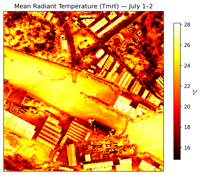
The calculation produces Tmrt and thermal comfort indices for each hour in the weather file, at every pixel in the grid.
Run 3. SOLWEIG Calculation from the Processing Toolbox:
- Prepared surface directory: the output directory from Step 3.
- Weather: select EPW weather file and choose the EPW file you downloaded in Step 2.
- Start date:
2021-07-01. End date:2021-07-02. This gives 48 hourly timesteps across two summer days. - Output Tmrt: checked. This is the primary output (Mean Radiant Temperature).
- Compute UTCI: checked. This derives the Universal Thermal Climate Index from Tmrt and the weather variables.
- Max shadow distance:
500metres. Bilbao sits in a river valley, so terrain shadows from surrounding hills can reach across the city floor. - Output directory: choose a folder (e.g.
bilbao_output).
Run.
The output directory will contain subdirectories for each component (tmrt, shadow, utci), with one GeoTIFF per timestep, plus summary grids in a summary folder.
This lesson uses building and vegetation heights but no land cover raster. SOLWEIG can also accept a land cover classification (grass, asphalt, water, etc.) to assign different emissivity and albedo values per surface type. Including land cover would improve the accuracy of ground surface temperatures and, in turn, Tmrt.
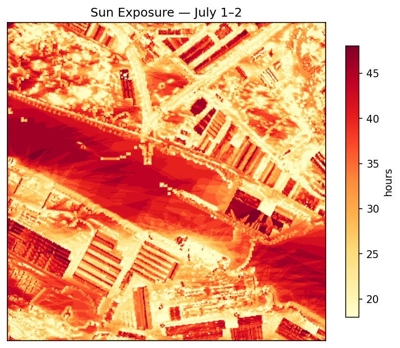
Step 5: Visualise the results
Navigate to the summary subdirectory in your output folder and load these into QGIS:
tmrt_mean.tif- Mean Radiant Temperature averaged over the full period.utci_mean.tif- Mean UTCI thermal comfort index.sun_hours.tif- Total sun exposure hours per pixel.
To style a raster: right-click the layer > Properties > Symbology. Change the render type to Singleband pseudocolor and pick a colour ramp (Magma or RdYlBu reversed work well for temperature data).
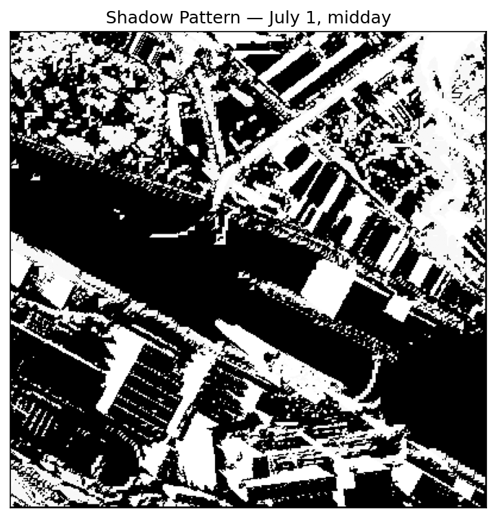
Step 6: Compare shadows across the day
Open the shadow subdirectory. Each file is named by timestamp (e.g. 20210701_0800.tif, 20210701_1200.tif).
Load a morning file (08:00) and a midday file (12:00). Shadow values are 0 (sunlit) and 1 (shaded); style with a black/white colour ramp. Compare the two.
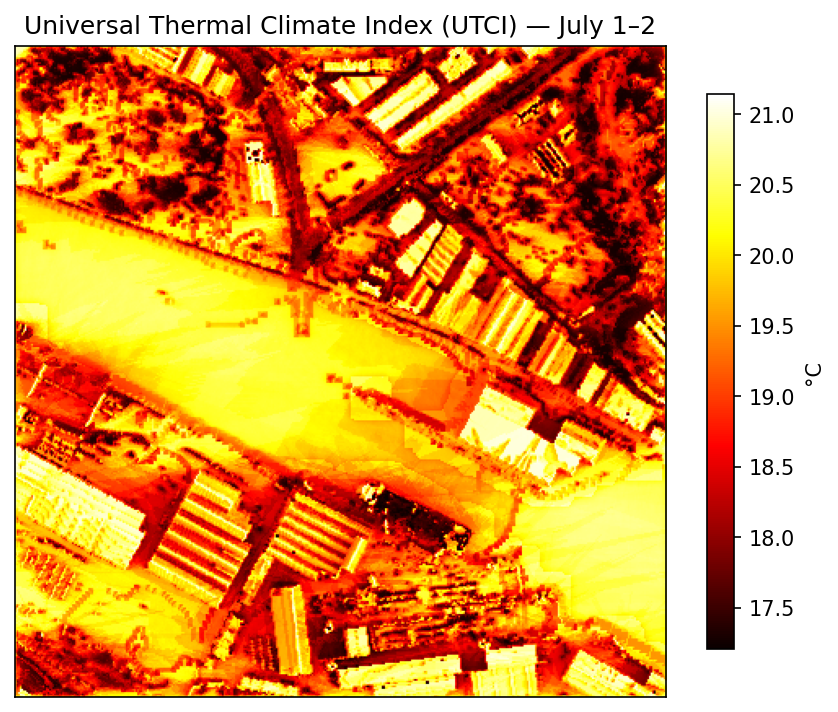
Step 7: Interpret UTCI
UTCI translates radiation, temperature, humidity, and wind into a single “feels like” temperature. The standard heat stress categories:
| UTCI (°C) | Stress category |
|---|---|
| > 46 | Extreme heat stress |
| 38 to 46 | Very strong heat stress |
| 32 to 38 | Strong heat stress |
| 26 to 32 | Moderate heat stress |
| 9 to 26 | No thermal stress |
| 0 to 9 | Slight cold stress |
Load utci_mean.tif and style it using the categories above. The summary folder also contains utci_hours_above_32_day.tif, which shows how many daytime hours each pixel exceeded 32°C (strong heat stress).
Next
Compare the outputs to the building heights and vegetation layers. The spatial patterns in Tmrt and UTCI are driven by the surface geometry you can see in the input rasters.