Hints & Solutions

Warning

Don’t look at the hints or solutions until first making a sincere effort to solve the steps yourself. If you really get stuck, take a look at the hints and (if necessary) the solution steps, but only as much as needed to get you going again.

Tip

There are many ways to solve most GIS workflows. It is OK if you use another way to achieve a similar outcome.

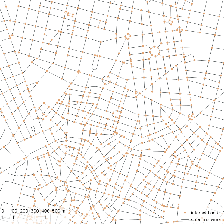
Hint 1: Generate intersections

The input streets layer contains LineString geometries, but we need Point geometries for the analysis. QGIS has a tool for extracting line intersections as points.

Solution

Open the Processing Toolbox and use the Line intersections tool. Use street_network for both the input and intersecting layers, then run. This will generate an Intersections layer.

Hint 2: Remove duplicate intersections

If you inspect the resultant intersections, you might notice that many of the intersections are duplicated where lines touched each other (since each line is extracted in turn). Remove duplicates before proceeding.

Solution

To remove the duplicates, use the Delete duplicate geometries tool and run it on the Intersections layer, which will generate the Cleaned layer, with the duplicates removed. This will bring your intersection features count down from around 213k to 30k.

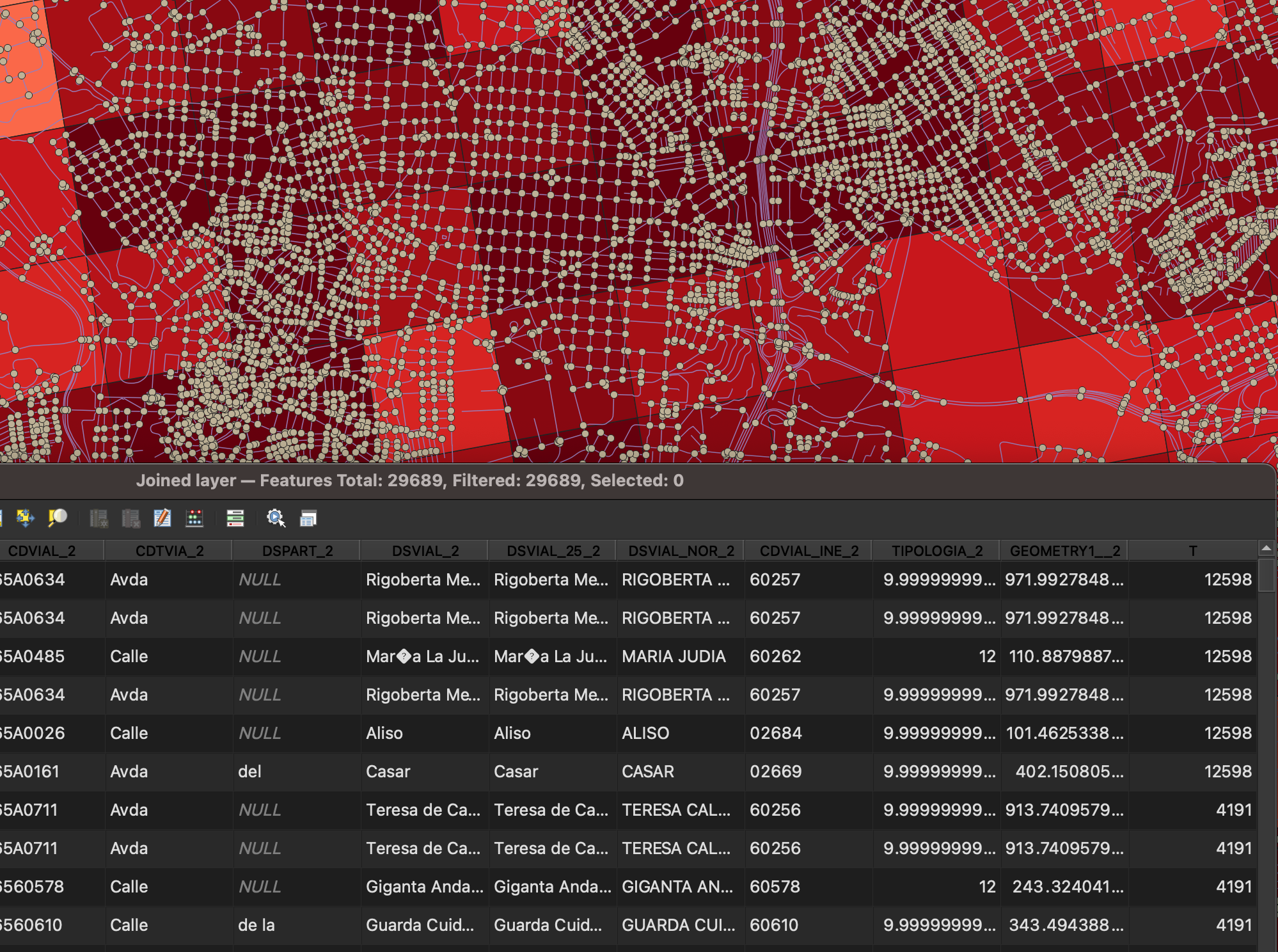
Hint 3: Join population data

Now we need to transfer the population density information from the grid to the intersections. To do so, join the population count for each census grid cell to any points contained by that cell.

Solution

Go to the Vector menu - Data Management Tools - Join Attributes by Location.
Use the Cleaned layer (from the previous step) as the “Join to features in” layer.
Use the eu_stat_clipped layer as the “By comparing to” layer.
Use intersect for the geometric predicate.
For “Fields to add”, select “T” (total population).
For “Join type”, select “Take attributes of the first matching feature”.

This will output a new Joined layer, which merges the intersections with a new attribute column T, which contains the per 1km2 population count for that location. Rename the layer to itx.

Hint 4: Buffering

We need to count the intersections and transport stops within 1km2 of each of the intersections. Instead of using 1km x 1km square cells, use a circular buffer with an area equivalent to 1km2 around each intersection. The radius comes from the area formula for a circle: r = sqrt(1,000,000 / pi), which gives roughly 564m. Create buffered Polygon geometries from the intersections.

Solution

Go to Vector > Geoprocessing Tools > Buffer. Select itx as the input layer and 565m as the buffer distance, then run. This will generate a new Buffered layer. You may want to turn off layer visibility!

Intersections, Buffers and Transport Points

Hint 5: Count intersections

Count the intersections (Points) contained by each of the buffered geometries (Polygons).

Solution

Go to Vector > Analysis Tools > Count Points in Polygon. Select the Buffered layer for the polygons and the itx layer as the points.
Set the Count field name to num and run.
This will generate a Count layer, but rename it to itx_counts.

Hint 6: Prepare transport stops

From the madrid_infrast layer, extract only the transport stops.

Solution

Open the Processing Toolbox and use Extract by Expression on the madrid_infrast layer with the following expression:

"class" = 'bus_stop'
  OR "class" = 'railway_station'
  OR "class" = 'subway_station'

This will create a new Matching features layer containing only transport stops, leaving the original layer untouched.

Hint 7: Count transport stops

Count the transport stops (Points) contained by each of the buffered geometries (Polygons).

Solution

Use Count Points in Polygon once again, this time reusing the Buffered layer but counting the extracted transport stops layer instead.
Set the Count field name to num and run.
This will generate a Count layer, but rename it to transport_counts

Hint 8: Joins

Join the derived itx_counts and transport_counts layers back into the itx layer. In Hint 3, we used a spatial join (matching by location). This time we need an attribute join (matching by a shared field), since the layers already share the same features in the same order.

Solution

Open the layer properties for the itx layer.
Go to the Joins view then add a join for itx_counts, using the fid fields for matching. Select the Joined fields checkbox and select the num field. This will join the count of intersections data back into the original itx layer.
Repeat for transport_counts, once again only joining the num field.
Export itx to madrid_joined.gpkg (with a layer name of madrid_joined). This step is important: layer property joins in QGIS are virtual. They only exist while the project is open with the source layers present. Exporting makes the joined fields permanent.

Hint 9: Setting the column names

Rename the attribute column names to those specified by the task.

Solution

Double click the madrid_joined layer in the Layers panel.
Click the Fields tab.
Toggle editing mode.
Rename (if necessary) your population count attribute to pop_km2.
Rename (if necessary) your intersection count attribute to itx_num.
Rename (if necessary) your transport count attribute to transport_num.

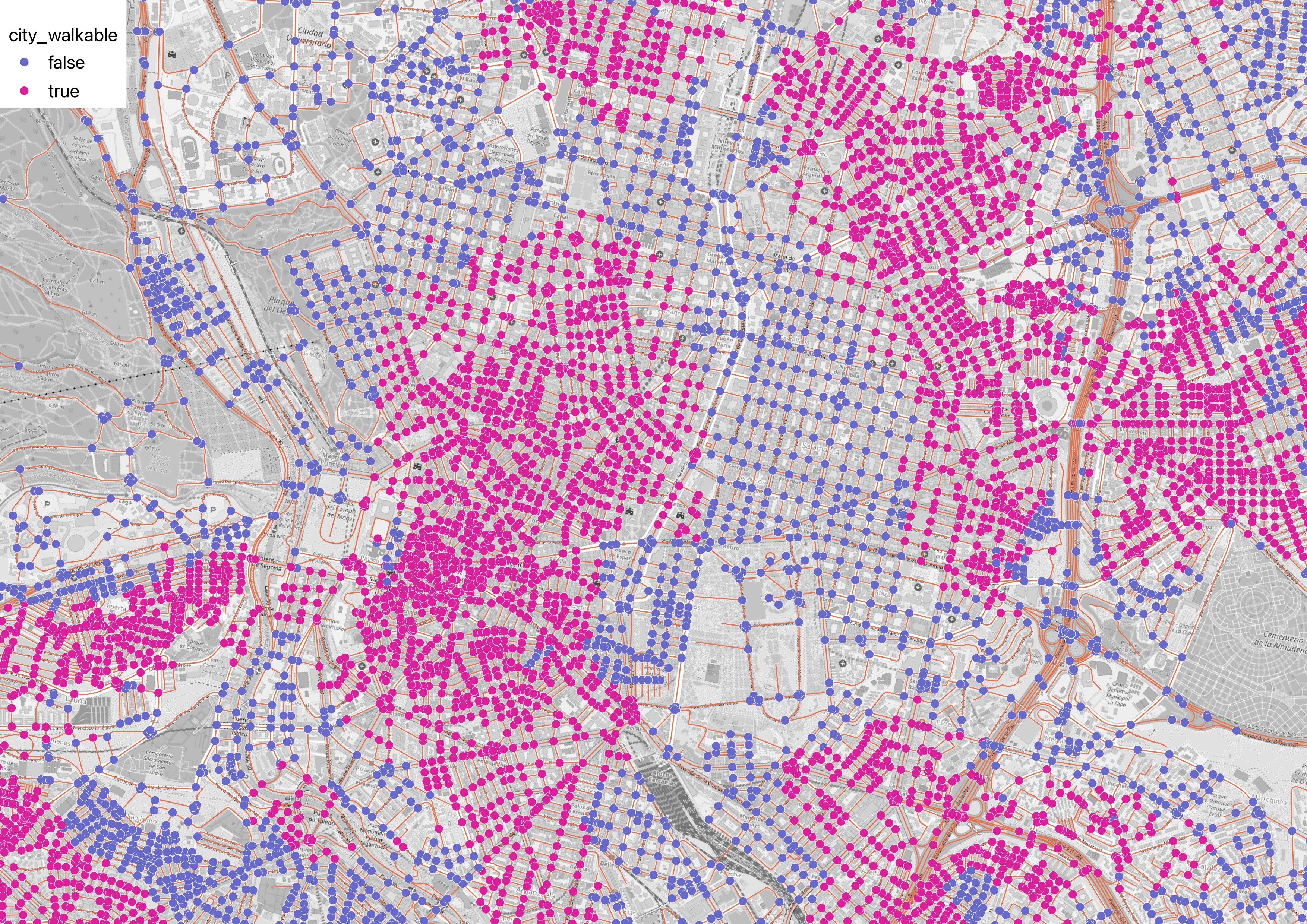
Hint 10: Setting walkability

Set the is_walkable attribute based on the walkability thresholds.

Solution

Open the Attribute Table and click the Field Calculator button (abacus icon).
Create a new boolean column called is_walkable using the following expression. Double-check the column names match.

if(
  "pop_km2" >= 5700
    AND "itx_num" >= 100
    AND "transport_num" >= 28,
  true,
  false
)

Save and toggle editing, then export as madrid_walkable.gpkg with a layer name of madrid_walkable.