Spatial Analysis
Spatial operations examine how features relate in space. You can ask questions like: which polygons overlap? What falls within a given distance of something? Where do two datasets intersect? These geometric relationships let you answer questions that attributes alone cannot.
This section covers the core spatial operations you’ll use repeatedly:
- Buffering: Expanding geometries by a given distance (e.g., “within 15m of a street”)
- Dissolve: Merging multiple features into one
- Difference: Subtracting one layer’s geometry from another
- Select by Location: Choosing features based on their spatial relationship to another layer
- Joins: Connecting attributes from one layer to another based on spatial relationships
For this section, you’ll need the madrid_nbhds.gpkg, street_network.gpkg, prems_food_bev.gpkg, and prems_cafeteria.gpkg files. The first two are on the datasets page. The last two you created in the previous section.
Spatial predicates define relationships between geometries: Intersects, Contains, Within, Touches, Equals, Overlaps. When you use “Select by Location”, you’re choosing which predicate to apply. These relationships are formally defined but the visual examples below are more useful than the formal definitions.
See the below links for visual examples:
Approximating Blocks
We have a blocks dataset, but what if we needed to approximate blocks ourselves? One approach: take a city boundary polygon, buffer the streets to give them width, then subtract the streets from the boundary. What remains are the approximate block shapes.
This exercise chains multiple spatial operations together: dissolve, select by location, buffer, and difference.
Step 1: Dissolving Neighbourhoods
First, we’ll Dissolve the neighbourhoods to merge them into a single Polygon for the whole of Madrid.
- Select
Vector→Geoprocessing Tools→Dissolveand check that themadrid_nbhdslayer is selected as Input Layer. - Click
Runand close the window once done.
This adds a temporary layer called Dissolved with merged neighbourhood geometries.
- Remove
madrid_nbhdsfrom the Layers panel. - Right-click and rename the new
Dissolvedlayer tomadrid.
Step 2: Select by Intersection
We need to Buffer the streets LineString geometries. But first, we’ll select only streets inside of Madrid since those outside of the boundary are not necessary and will just slow things down.
- Go to
Vector→Research Tools→Select by Location - Select features from the
street_networklayer. - Compare to the
madridlayer (the Madrid boundary). - Use
intersectfor the geometric predicate. - Select
creating new selectionfor selection mode. - Click
Runand close the window once done.
Step 3: Buffering Streets
All streets that Intersect the Madrid boundary are now selected. We’ll use these for the next step, where we perform the Buffer.
- Select
Vector→Geoprocessing Tools→Bufferand check that thestreet_networklayer is selected. - Check the box for “Selected features only”.
- Use 7m for the buffer distance. This approximates a typical street half-width; the buffer extends from the centreline, so 7m on each side gives roughly 14m total street width. Adjust based on your needs.
- Do not select the option to automatically dissolve the result. We’ll do this manually for now.
- Click
Runand close the window once done.
Step 4: Dissolving Streets
If you inspect the new Buffered layer, you’ll see that each LineString has been buffered into Polygon geometries. Let’s go ahead and Dissolve these as well.
- Select
Vector→Geoprocessing Tools→Dissolveand check that theBufferedlayer is selected. - This time, we’ll save the output to a file by selecting the dropdown next to the lowermost text field and selecting
Save to GeoPackagethen save it asstreets_dissolved. When prompted, usestreets_dissolvedfor the GeoPackage Layer name. - Click
Runand close the window once done. - Remove the layer
Bufferedfrom the Layers panel, since it is no longer needed.
Step 5: Differencing Streets from Boundary
We now need to perform a Difference so that the buffered streets are subtracted from the Madrid boundary, giving us the approximated block outlines.
- Select
Vector→Geoprocessing Tools→Difference - Select the
madridlayer for the input and thestreets_dissolvedfor the overlay. - Save the output to a file by selecting the dropdown next to the lowermost text field and selecting
Save to GeoPackagethen save it asblock_outlines. When prompted, useblock_outlinesfor the GeoPackage Layer name. - Click
Runand close the window once done. - Remove
streets_dissolvedfrom the Layers panel.
Step 6: Exploding Multipart to Singleparts
We now have a giant MultiPolygon which we need to explode into separate Polygons, one for each block.
- Go to
Vector→Geometry Tools→Multipart to Singleparts - Check that the
block_outlinesinput layer is selected. - Save the output to a file by selecting the dropdown next to the lowermost text field and selecting
Save to GeoPackagethen save it asbasic_blocks. When prompted, usebasic_blocksfor the GeoPackage Layer name. - Click
Runand close the window once done. - Remove
block_outlinesfrom the Layers panel.
The resultant basic_blocks layer now contains approximated blocks. Note that you’ve used a combination of different spatial operations, including Buffer, Dissolve, Intersect, and Difference.
Joins
Joins connect information from one layer to another for analysis or visualisation.
Join Types
There are two general approaches to Joins in GIS:
- Joins based on a shared data attribute: a dataset can be merged with a different dataset as long as both datasets share common identifiers. For example, a GeoPackage layer with Polygons postcode boundaries contains a unique identifier in the form of each postcode. A different CSV dataset containing census demographics for each postcode can therefore be merged into the Polygon layer by matching against the postcode identifiers.
- Spatial Joins based on spatial relationships: When working with two spatial datasets, it is possible to connect data purely based on the spatial relationships between the layers. For example, if a Polygon layer contains neighbourhood boundaries and a Points layer contains pollution sensors, then a spatial Join can be used to calculate average pollution levels by neighbourhood.
Cardinality
In the simplest case, a Join connects one feature to one other feature: a one-to-one relationship. More often, one feature connects to multiple features. A postcode boundary might contain dozens of pollution sensors: a one-to-many relationship. There are also many-to-many relationships, though these are less common in typical GIS workflows.
Joins in QGIS
The full power of these methods is available in spatial databases such as PostGIS. In the case of QGIS, the use of Joins and cardinality is implicit with functionality bundled in tools, which we will use during this and the next lesson. There are certain constraints depending on the tool:
Vector→Research Tools→Select by Location(which we’ve already used above) allows you to select features based on their relationship to features in another layer.Vector→Analysis Tools→Count Points in Polygonuses an implicit one-to-many Join to count Points falling within Polygons.- The QGIS Joining Features Between Layers functionality is based on a one-to-one relationship between matching attributes and describes a process for how duplicate entries are resolved.
Vector→Data Management Tools→Join Attributes By Location (summary)(available in the Processing Toolbox, which we’ll use in the next lesson) aggregates attributes from one spatial layer based on its relationship with another, enabling statistical summaries (e.g., sum, mean, count) in one-to-many analyses. For example, averaging pollution sensor data by neighbourhood boundaries.
Cafeterias by Street
Let’s use spatial analysis to answer a question: which streets in Madrid have access to the most Cafeterias?
We have a streets layer and we’ve already prepared a premises layer for Cafeterias, so we need to:
- Buffer the streets by a selected distance.
- Count the number of cafeterias within the buffers.
- Join the resultant counts information from the buffered counts back into the original streets layer.
- Visualise the results.
For a clean workspace, remove layers you don’t need (keep basic_blocks if you want it for the challenge later). Add the street_network and prems_cafeteria layers.
Step 1: Buffering Streets
This time, we’ll buffer streets by 15m (capturing cafeterias roughly within that distance of each street) without dissolving, so each street keeps its own buffer.
- Select
Vector→Geoprocessing Tools→Bufferand check that thestreet_networklayer is selected. - Use 15m for the buffer distance.
- Do not select the option to automatically dissolve the result.
- Click
Runand close the window once done.
Step 2: Count Points in Polygon
Now we need to count the premises points falling within each of the street buffers.
- Select
Vector→Analysis Tools→Count Points in Polygon. - Check that the
Bufferedlayer is selected for Polygons andprems_cafeteriafor Points. - Click
Runand close the window once done. - Remove
Bufferedfrom the Layers panel.
This creates a new layer called Count which contains a new attribute called NUMPOINTS containing the counts of Cafeterias falling within each Polygon.
Step 3: Join the Data
Joins are a way to connect information from one layer to another based on a matching identifier. We’ve counted the number of points contained by the buffers and we need a way to connect this information from the Count layer back into the original street_network layer for visualisation purposes.
Since the layers with the buffered counts originated from the streets layer, the original attributes were automatically copied across when creating the derivative buffers and counts. We can therefore use the matching feature identifiers to connect this information back into the original layer.
- Double-click the
street_networklayer. - Select the
Joinstab. - Click the plus button.
- Select the
Countlayer. - Select
fid(feature ID) for both the Join and Target fields. This will match rows fromCountinto rows withinstreet_networkwhere thefidvalues match. - Click
OKand close the dialogue box. - Deselect the
Countlayer in the Layers panel so that it doesn’t obscure the streets layer.
The new NUMPOINTS data is now connected (Joined) into the original street_network layer. Open the Attribute Table where you’ll see attribute columns from the Count layer, prepended with Count_.
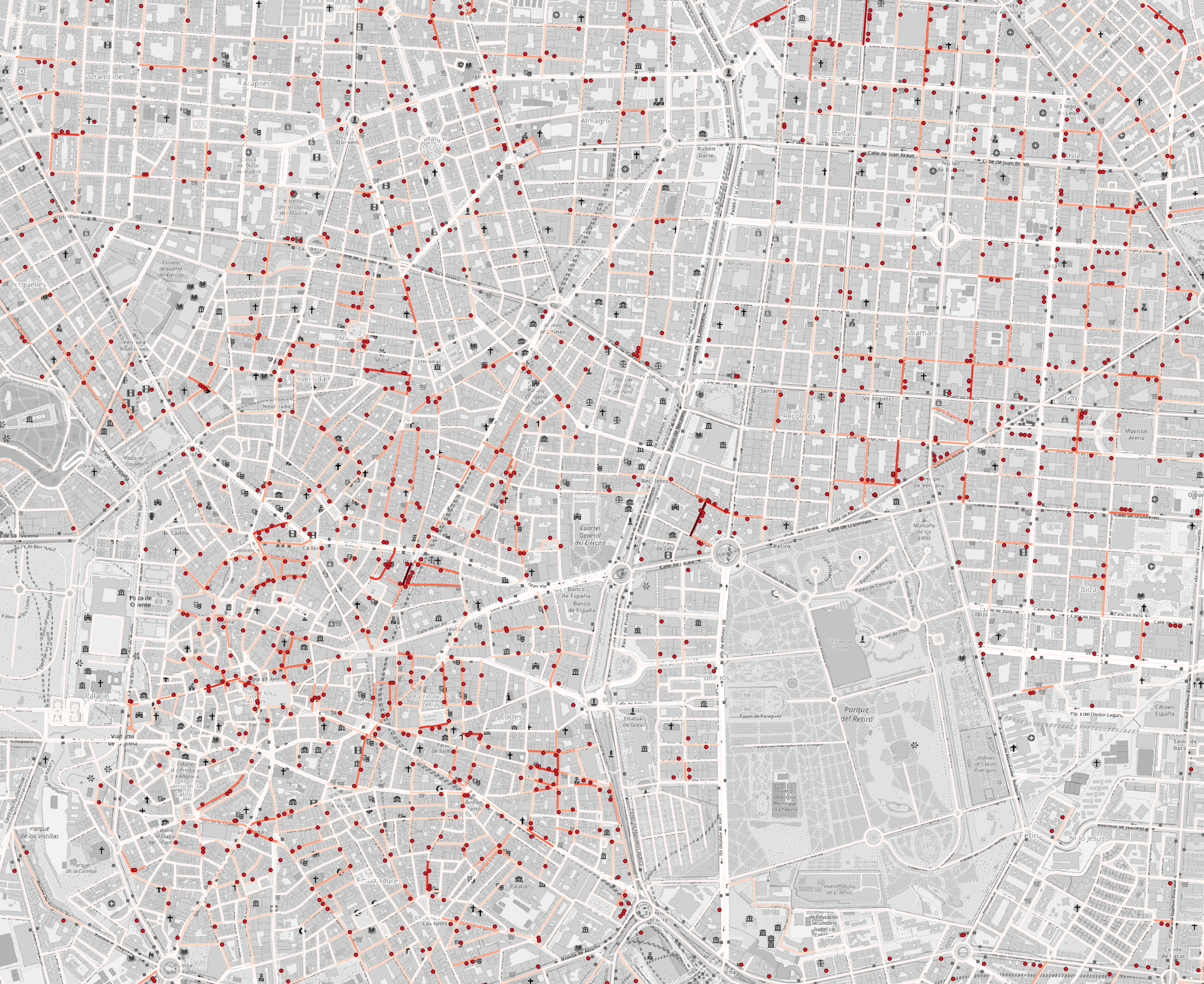
Step 4: Visualise
The Count_NUMPOINTS column now shows cafeteria counts per street. Style it with a graduated colour scheme to see the distribution.
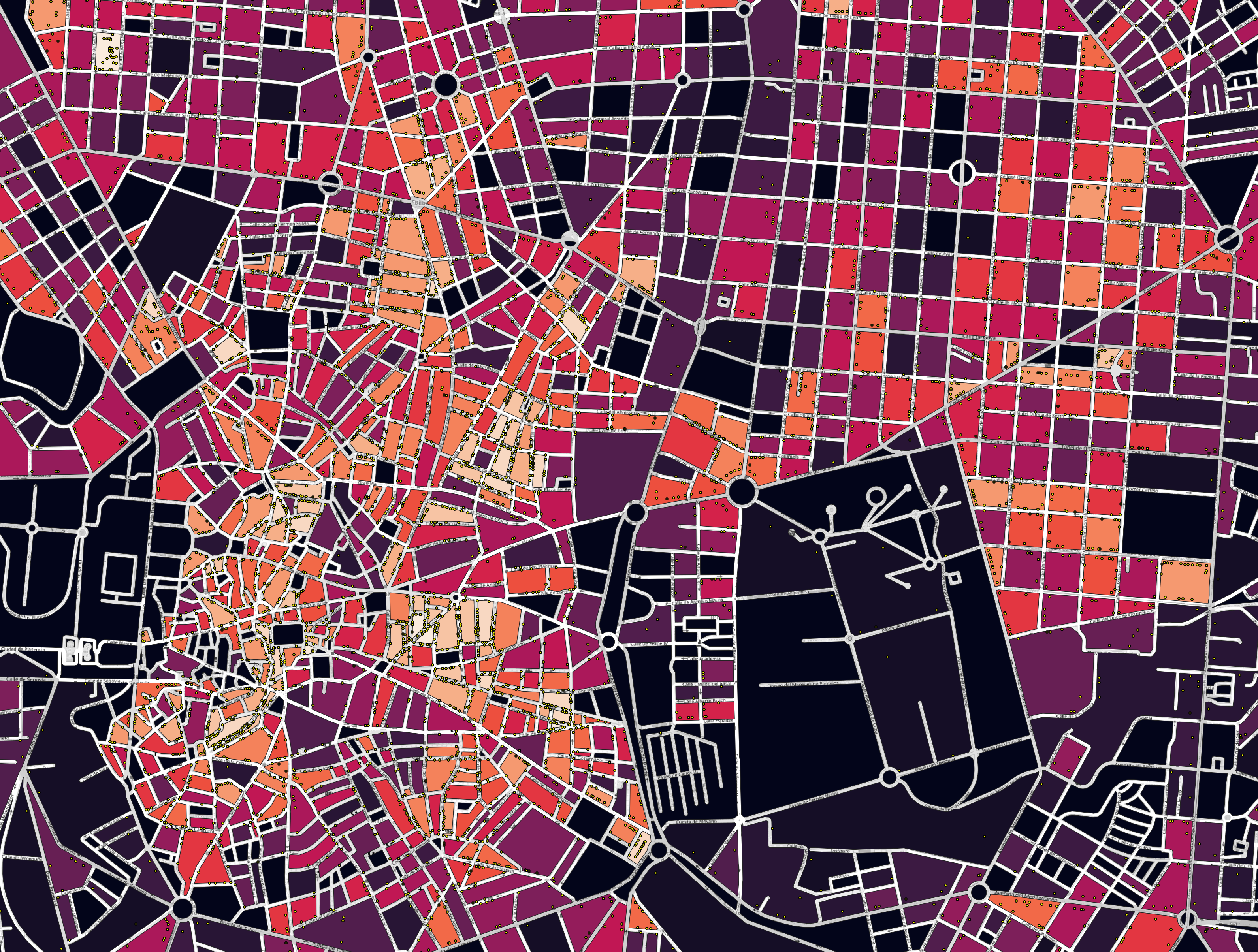
Challenge: Landuse Counts by Block
This challenge combines everything from this lesson: buffering, counting, joins, expressions, and styling. It has multiple steps, so work through it carefully.
- Using your new
basic_blockslayer, export a copy calledbasic_blocks_copyso that changes are not made to the original. - Using
basic_blocks_copy, discard all blocks with perimeters less than 50m. - Using the
prems_food_bevlayer saved previously, count the number of food and beverage locations inside or within 5m of each block (not all landuses are precisely contained by a block). - Add a column to the Attribute Table called
food_bev_perim_kmcontaining the count of Food and Beverage locations per km length of the block perimeter. - Visualise the results.
- If you encounter geometry validity errors, use the
Vector→Geometry Tools→Check Validitytool. Then use the derivativeValid outputlayer. - There is a
$perimeterexpression which returns the Polygon perimeter.
Step 1
- Open the Attribute Table for the
basic_blocks_copylayer and open the Field Calculator. - Create a new column called
perimof aDecimal Number (real)type, using$perimeterfor the expression. - Select features using the expression
"perim" < 50. - Delete selected rows.
- Toggle edit mode and save.
Step 2
- Select
Vector→Geoprocessing Tools→Bufferand check that thebasic_blocks_copylayer is selected. - Use 5m for the buffer distance.
- Do not select the option to automatically dissolve the result.
- Click
Runand close the window once done.
Step 3
This step might be unnecessary for you but is included in-case the previous steps have given you “invalid” geometries.
- Select
Vector→Geometry Tools→Check Validityand check that theBufferedlayer is selected. - Click
Runand close the window once done.
Step 4
- Select
Vector→Analysis Tools→Count Points in Polygon. - For Polygons, select
Valid output(if you ran Step 3) orBuffered(if you skipped Step 3). - For Points, select
prems_food_bev. - Click
Runand close the window once done.
Step 5
- Open the Attribute Table for the new
Countlayer and open the Field Calculator. - Create a new column called
food_bev_perim_kmof aDecimal Number (real)type, using"NUMPOINTS" / ("perim" / 1000)for the expression. - Save the edits.
Step 6
- Double-click the
basic_blocks_copylayer. - Select the
Joinstab. - Click the plus button.
- Select the
Countlayer. - Select
fid(feature ID) for both the Join and Target fields. - Click
OKand close the dialogue box.
Step 7
- Visualise the
basic_blocks_copylayer using aGraduatedstyle. Use theCount_food_bev_perim_kmcolumn.