# Uncomment to install geopandas
# !pip install geopandas

from shapely import geometry
import geopandas as gpdGeoPandas
geopandas extends pandas with built-in support for shapely geometries. Where shapely handles individual geometries, geopandas lets you work with thousands of them at once in a tabular format, performing spatial operations across entire columns and filtering rows by attribute data.
Note
As with numpy or pandas: follow along for now and the syntax will become familiar with practice.
Creating a GeoDataFrame
The core data structure is the GeoDataFrame: a pandas DataFrame with a geometry column.
To see how it works, we’ll create a grid of Point objects using a nested loop. The nested loop creates every combination of x and y, so 4 x values and 4 y values produce 16 points.
x_coords = [0, 1, 2, 3]
y_coords = [0, 1, 2, 3]

collect_points = []

for x in x_coords:
  for y in y_coords:
    p = geometry.Point(x, y)
    collect_points.append(p)

print('num points:', len(collect_points))
num points: 16Now create a GeoDataFrame from the list of points. We have no attribute data (data=None) and no formal coordinate reference system (crs=None):
df = gpd.GeoDataFrame(
  data=None,
  geometry=collect_points,
  crs=None
)

df.head()| geometry | |
|---|---|
| 0 | POINT (0 0) |
| 1 | POINT (0 1) |
| 2 | POINT (0 2) |
| 3 | POINT (0 3) |
| 4 | POINT (1 0) |
GeoDataFrames have built-in plotting through the plot() method:
df.plot()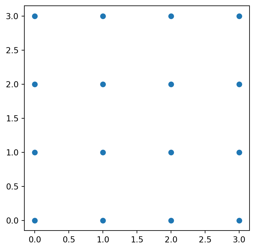
The geometry column is a GeoSeries, which supports shapely operations across all rows at once. For example, buffer() buffers every geometry in the column:
df.geometry = df.geometry.buffer(0.6)
df.head()| geometry | |
|---|---|
| 0 | POLYGON ((0.6 0, 0.59711 -0.05881, 0.58847 -0.... |
| 1 | POLYGON ((0.6 1, 0.59711 0.94119, 0.58847 0.88... |
| 2 | POLYGON ((0.6 2, 0.59711 1.94119, 0.58847 1.88... |
| 3 | POLYGON ((0.6 3, 0.59711 2.94119, 0.58847 2.88... |
| 4 | POLYGON ((1.6 0, 1.59711 -0.05881, 1.58847 -0.... |
df.plot()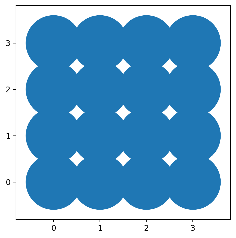
The GeoSeries has attributes like area and centroid that you can use to populate new columns:
df['area'] = df.geometry.area
df.round(2).head()| geometry | area | |
|---|---|---|
| 0 | POLYGON ((0.6 0, 0.59711 -0.05881, 0.58847 -0.... | 1.13 |
| 1 | POLYGON ((0.6 1, 0.59711 0.94119, 0.58847 0.88... | 1.13 |
| 2 | POLYGON ((0.6 2, 0.59711 1.94119, 0.58847 1.88... | 1.13 |
| 3 | POLYGON ((0.6 3, 0.59711 2.94119, 0.58847 2.88... | 1.13 |
| 4 | POLYGON ((1.6 0, 1.59711 -0.05881, 1.58847 -0.... | 1.13 |
df['x'] = df.geometry.centroid.x
df['y'] = df.geometry.centroid.y

df.round(2).head()| geometry | area | x | y | |
|---|---|---|---|---|
| 0 | POLYGON ((0.6 0, 0.59711 -0.05881, 0.58847 -0.... | 1.13 | -0.0 | -0.0 |
| 1 | POLYGON ((0.6 1, 0.59711 0.94119, 0.58847 0.88... | 1.13 | -0.0 | 1.0 |
| 2 | POLYGON ((0.6 2, 0.59711 1.94119, 0.58847 1.88... | 1.13 | 0.0 | 2.0 |
| 3 | POLYGON ((0.6 3, 0.59711 2.94119, 0.58847 2.88... | 1.13 | 0.0 | 3.0 |
| 4 | POLYGON ((1.6 0, 1.59711 -0.05881, 1.58847 -0.... | 1.13 | 1.0 | 0.0 |
As with pandas, you can filter rows by condition:
filtered_df = df[df.x < 2]
filtered_df.plot()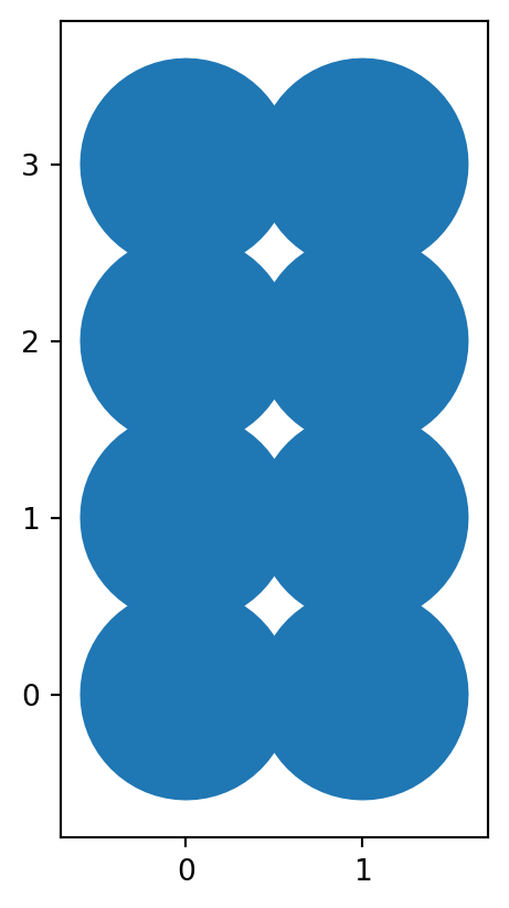
Approximating Blocks (Again!)
NoteData
Please download the following two data files and place them in your Colab folders. We’ll walk through an example in class:
TipFilepaths!
In Python notebooks, file-paths tell Python where to find and save files. They can be absolute (full path from the “root” directory) or relative (based on the working directory location). When you tell Python to load or save a file, you need to use an accurate file-path so that it looks in the correct location.
Absolute vs. Relative Paths
- Absolute → Full path from root – note leading slash:
/content/file.gpkg(inside acontentfolder)
- Relative → Based on the notebook’s location – note no leading slash:
data/file.gpkg(inside adatafolder)
We’ll replicate the Approximating Blocks exercise from the QGIS lesson, this time in Python.
import geopandas as gpdread_file() reads GeoPackage and other geospatial file formats directly. You may need to update the file path to match the file location on your system.
gdf_nbhds = gpd.read_file("../../data/madrid_nbhds/madrid_nbhds.gpkg")

print(gdf_nbhds.crs)
print(gdf_nbhds.crs.is_projected)
EPSG:25830
TrueAlways check the CRS. Spatial operations based on metres will give wrong results if applied to geographic coordinates (degrees). If something seems off, CRS mismatch is the first thing to investigate.
gdf_nbhds.head()| CODDIS | NOMDIS | COD_BAR | NOMBRE | Shape_Leng | COD_DIS_TX | BARRIO_MAY | COD_DISBAR | NUM_BAR | BARRIO_MT | COD_DISB | geometry | |
|---|---|---|---|---|---|---|---|---|---|---|---|---|
| 0 | 1 | Centro | 011 | Palacio | 0.0 | 01 | PALACIO | 11 | 1 | PALACIO | 1-1 | MULTIPOLYGON (((440112.785 4474645.921, 440078... |
| 1 | 1 | Centro | 012 | Embajadores | 0.0 | 01 | EMBAJADORES | 12 | 2 | EMBAJADORES | 1-2 | MULTIPOLYGON (((440277.382 4473980.839, 440368... |
| 2 | 1 | Centro | 013 | Cortes | 0.0 | 01 | CORTES | 13 | 3 | CORTES | 1-3 | MULTIPOLYGON (((440780.52 4474528.375, 440907.... |
| 3 | 1 | Centro | 014 | Justicia | 0.0 | 01 | JUSTICIA | 14 | 4 | JUSTICIA | 1-4 | MULTIPOLYGON (((440991.949 4474492.423, 440907... |
| 4 | 1 | Centro | 015 | Universidad | 0.0 | 01 | UNIVERSIDAD | 15 | 5 | UNIVERSIDAD | 1-5 | MULTIPOLYGON (((440517.952 4474758.368, 440476... |
gdf_nbhds.plot()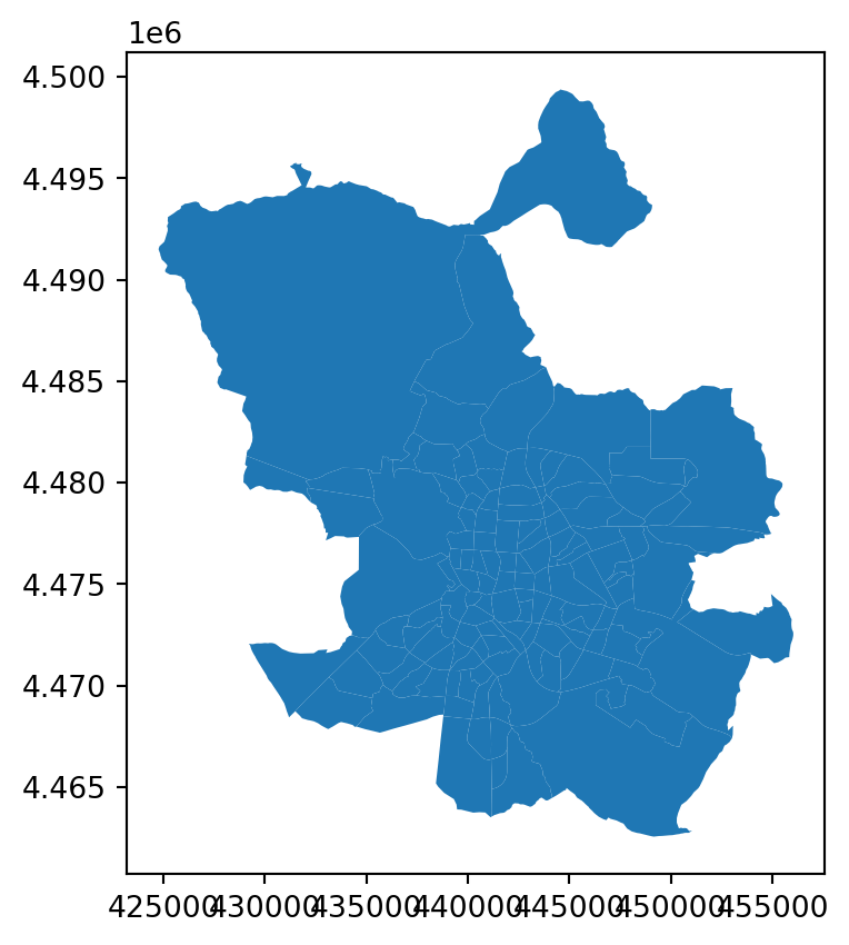
dissolve() merges all geometries into a single row, giving us a unified Madrid outline:
madrid_bounds_geom = gdf_nbhds.dissolve()

print(type(madrid_bounds_geom))
madrid_bounds_geom
<class 'geopandas.geodataframe.GeoDataFrame'>| geometry | CODDIS | NOMDIS | COD_BAR | NOMBRE | Shape_Leng | COD_DIS_TX | BARRIO_MAY | COD_DISBAR | NUM_BAR | BARRIO_MT | COD_DISB | |
|---|---|---|---|---|---|---|---|---|---|---|---|---|
| 0 | POLYGON ((441182.611 4463570.002, 441178.708 4... | 1 | Centro | 011 | Palacio | 0.0 | 01 | PALACIO | 11 | 1 | PALACIO | 1-1 |
Next, read the street network:
madrid_streets = gpd.read_file("../../data/madrid_streets/street_network.gpkg")

madrid_streets.head()| clased | nombre | geometry | |
|---|---|---|---|
| 0 | Autopista libre / autovía | M-406 | LINESTRING (437440 4460857, 437460 4460868, 43... |
| 1 | Carretera convencional | M-406 | LINESTRING (437438 4460861, 437472 4460878) |
| 2 | Urbano | FUERZAS ARMADAS (DE LAS) | LINESTRING (438131 4461473, 438133 4461461, 43... |
| 3 | Urbano | FUERZAS ARMADAS (DE LAS) | LINESTRING (438023 4461398, 438058 4461407, 43... |
| 4 | Carretera convencional | M-406 | LINESTRING (438181 4461468, 438177 4461465, 43... |
madrid_streets.plot()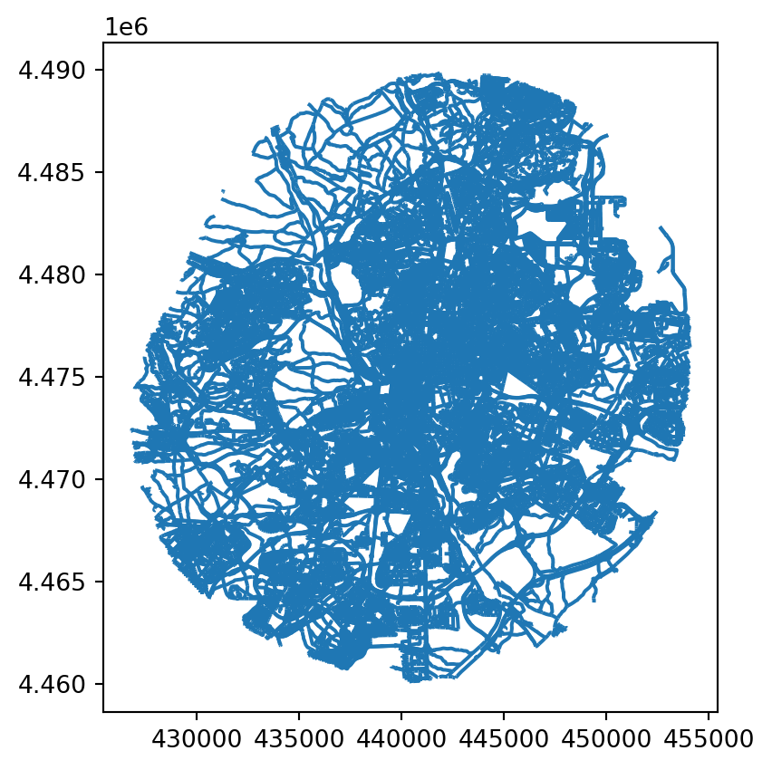
Confirm both files share the same CRS:
print(gdf_nbhds.crs == madrid_streets.crs)TrueUse copy() to keep an unaltered version of the streets for later:
madrid_streets_buff = madrid_streets.copy()Buffer the streets by 7 metres:
madrid_streets_buff.geometry = madrid_streets_buff.geometry.buffer(7)

madrid_streets_buff.head()| clased | nombre | geometry | |
|---|---|---|---|
| 0 | Autopista libre / autovía | M-406 | POLYGON ((437456.036 4460873.809, 437467.519 4... |
| 1 | Carretera convencional | M-406 | POLYGON ((437468.87 4460884.261, 437469.498 44... |
| 2 | Urbano | FUERZAS ARMADAS (DE LAS) | POLYGON ((438139.905 4461462.151, 438139.985 4... |
| 3 | Urbano | FUERZAS ARMADAS (DE LAS) | POLYGON ((438055.106 4461413.484, 438098.713 4... |
| 4 | Carretera convencional | M-406 | POLYGON ((438181.973 4461459.98, 438169.561 44... |
Dissolve the buffered streets into a single geometry:
madrid_streets_buff = madrid_streets_buff.dissolve()

print(type(madrid_streets_buff))
madrid_streets_buff.head()
<class 'geopandas.geodataframe.GeoDataFrame'>| geometry | clased | nombre | |
|---|---|---|---|
| 0 | MULTIPOLYGON (((428560.407 4466612.498, 428560... | Autopista libre / autovía | M-406 |
madrid_streets_buff.plot()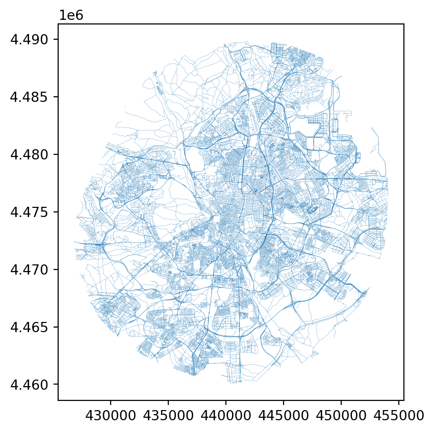
Now subtract the buffered streets from the Madrid boundary using difference(), which leaves the block outlines:
madrid_bounds_diff = madrid_bounds_geom.difference(madrid_streets_buff)

print(type(madrid_bounds_diff))
madrid_bounds_diff.head()
<class 'geopandas.geoseries.GeoSeries'>0 MULTIPOLYGON (((441175.474 4463566.211, 441169...
dtype: geometryThe output is a GeoSeries, so convert it back to a GeoDataFrame:
madrid_bounds_diff_gdf = gpd.GeoDataFrame(
    data=None, geometry=madrid_bounds_diff, crs=madrid_bounds_diff.crs
)

print(type(madrid_bounds_diff_gdf))
madrid_bounds_diff_gdf.head()
<class 'geopandas.geodataframe.GeoDataFrame'>| geometry | |
|---|---|
| 0 | MULTIPOLYGON (((441175.474 4463566.211, 441169... |
madrid_bounds_diff_gdf.plot()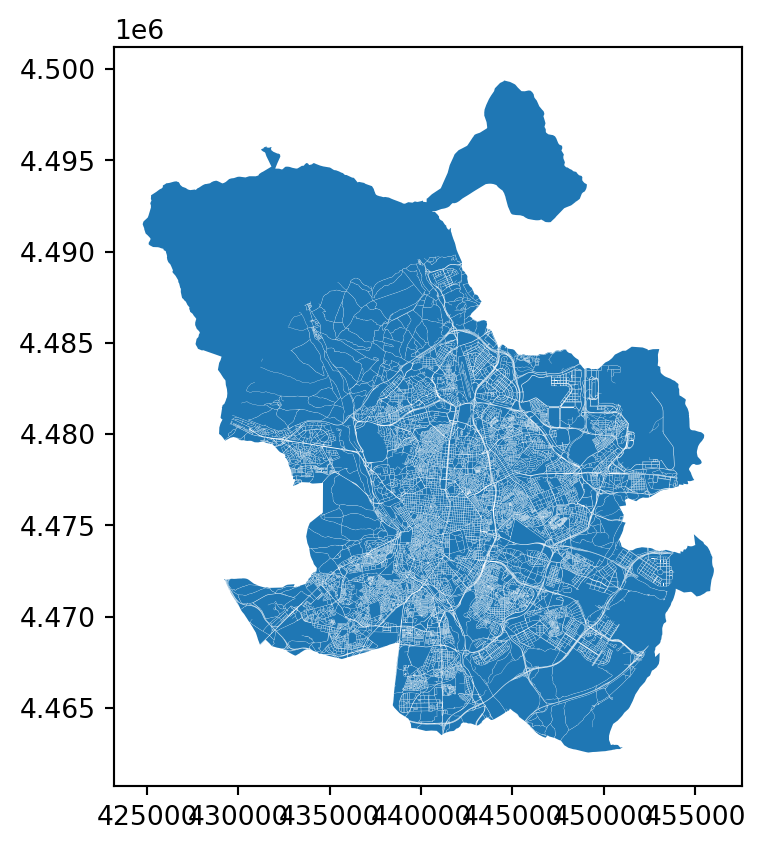
The result is a single MultiPolygon. explode() splits it into individual Polygon rows:
madrid_blocks = madrid_bounds_diff_gdf.explode(ignore_index=True)

madrid_blocks.head()| geometry | |
|---|---|
| 0 | POLYGON ((441175.474 4463566.211, 441169.34 44... |
| 1 | POLYGON ((439674.632 4463894.481, 439465.293 4... |
| 2 | POLYGON ((439376.065 4464270.402, 439435.048 4... |
| 3 | POLYGON ((439366.716 4464290.111, 439391.932 4... |
| 4 | POLYGON ((439352.399 4464320.295, 439364.88 44... |
madrid_blocks.plot()
Add an area column for plotting:
madrid_blocks["area"] = madrid_blocks.geometry.area
madrid_blocks.head()| geometry | area | |
|---|---|---|
| 0 | POLYGON ((441175.474 4463566.211, 441169.34 44... | 465529.325792 |
| 1 | POLYGON ((439674.632 4463894.481, 439465.293 4... | 127887.327516 |
| 2 | POLYGON ((439376.065 4464270.402, 439435.048 4... | 5048.640303 |
| 3 | POLYGON ((439366.716 4464290.111, 439391.932 4... | 1070.895497 |
| 4 | POLYGON ((439352.399 4464320.295, 439364.88 44... | 4982.779048 |
This time we’ll colour by area, set the colour range, and zoom into an area of interest:
ax = madrid_blocks.plot(column="area", cmap="inferno_r", vmin=0, vmax=20000)
ax.set_xlim(438000, 438000 + 4000)
ax.set_ylim(4472000, 4472000 + 4000)
ax.axis(False)  # hides the axis ticks and borders
(np.float64(438000.0),
np.float64(442000.0),
np.float64(4472000.0),
np.float64(4476000.0))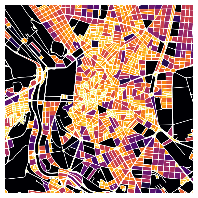
Bonus: Filtering
DataFrames can be filtered by attribute values. Here we’ll categorise streets by length, replicating the QGIS exercise.
First, compute percentile thresholds using numpy’s percentile():
import numpy as np

p_25 = np.percentile(madrid_streets.geometry.length, 25)
p_45 = np.percentile(madrid_streets.geometry.length, 45)
p_55 = np.percentile(madrid_streets.geometry.length, 55)
p_75 = np.percentile(madrid_streets.geometry.length, 75)

print(p_25, p_45, p_55, p_75)
28.635642126552707 51.78717834081825 66.63922355184319 108.1025473117499Now assign each street a category code (1-5) based on its length. The loc[] indexer selects rows matching a condition and assigns a value to the specified column (creating it if needed):
madrid_streets.loc[madrid_streets.geometry.length >= p_75, "cat_code"] = 5
madrid_streets.loc[madrid_streets.geometry.length < p_75, "cat_code"] = 4
madrid_streets.loc[madrid_streets.geometry.length < p_55, "cat_code"] = 3
madrid_streets.loc[madrid_streets.geometry.length < p_45, "cat_code"] = 2
madrid_streets.loc[madrid_streets.geometry.length < p_25, "cat_code"] = 1
madrid_streets.head()| clased | nombre | geometry | cat_code | |
|---|---|---|---|---|
| 0 | Autopista libre / autovía | M-406 | LINESTRING (437440 4460857, 437460 4460868, 43... | 2.0 |
| 1 | Carretera convencional | M-406 | LINESTRING (437438 4460861, 437472 4460878) | 2.0 |
| 2 | Urbano | FUERZAS ARMADAS (DE LAS) | LINESTRING (438131 4461473, 438133 4461461, 43... | 4.0 |
| 3 | Urbano | FUERZAS ARMADAS (DE LAS) | LINESTRING (438023 4461398, 438058 4461407, 43... | 5.0 |
| 4 | Carretera convencional | M-406 | LINESTRING (438181 4461468, 438177 4461465, 43... | 1.0 |
ax = madrid_streets.plot(column="cat_code", cmap="Spectral")
ax.set_xlim(438000, 438000 + 4000)
ax.set_ylim(4472000, 4472000 + 4000)
ax.axis(False)
(np.float64(438000.0),
np.float64(442000.0),
np.float64(4472000.0),
np.float64(4476000.0))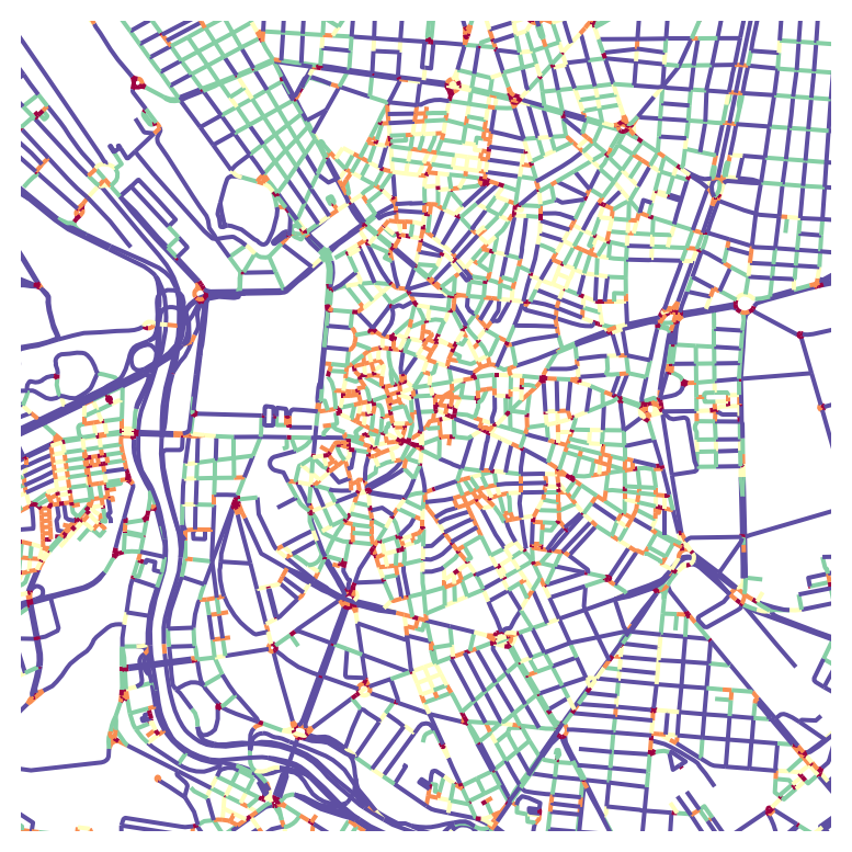
Tip
LLMs are good at helping with geopandas syntax. If you describe your GeoDataFrame structure (column names, types), you can ask how to filter, aggregate, or configure plot parameters.
Saving a GeoPandas File
Save GeoDataFrames to disk with to_file(). The resulting files can be opened in QGIS or other GIS software.
# uncomment and update file path to run
# madrid_blocks.to_file('../../temp/madrid_blocks_approx.gpkg')
# uncomment and update file path to run
# madrid_streets.to_file('../../temp/madrid_streets_cats.gpkg')There is more to geopandas than what we’ve covered here. Over the coming lessons we’ll use it more extensively for geospatial analysis.