Data Attributes
Attributes turn map features into useful information. A basic map shows where things are; attributes tell you what they are. For example, a building footprint can store its height (a number), its construction date (a date), and its current use (text). Each attribute has a data type that determines what values it can hold.
In QGIS, every point, line, or polygon stores attributes in its Attribute Table. You can filter features by their characteristics, run targeted analysis, or style maps based on attribute values.
This section covers viewing, filtering, and editing attributes to answer real-world questions about spatial data.
For these steps, you’ll need to download the madrid_premises.gpkg and street_network.gpkg datasets linked on the datasets page. Add these to your QGIS project.
Attribute Table
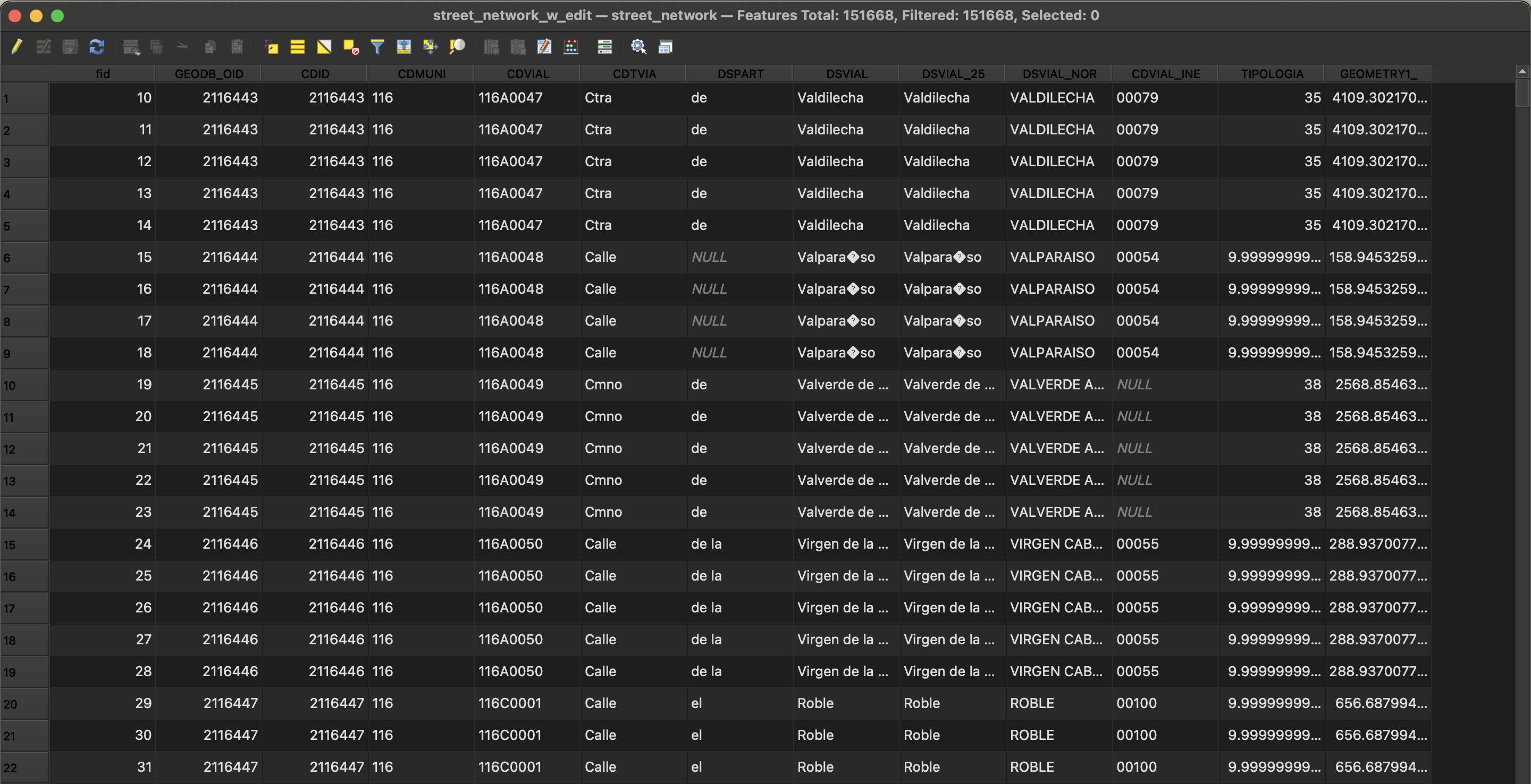
Right-click any layer in the Layers Panel and select “Open Attribute Table” (or click the icon in the toolbar). This opens a spreadsheet-like interface showing all data associated with your spatial features. Each row represents one feature (a street, a premises location), and each column represents a different attribute.
This works like a spreadsheet, except every row links to a geographic feature on your map. When you select a row in the Attribute Table, QGIS highlights the corresponding feature on the map, and vice versa.
Let’s open an Attribute Table for the streets data and look at its key components:
- The menu bar at the top provides tools for selecting, filtering, and editing your data
- The field names (column headers) show what type of information is stored
- The row numbers on the left correspond to unique features
- The cell contents store the actual values for each attribute
The Attribute Table in QGIS offers several useful tools for organising and navigating your data.
- You can sort rows by clicking any column header - click once to sort in ascending order, and again to sort in descending order. This is particularly useful when you want to quickly find the highest or lowest values in a numeric field, or organise names alphabetically.
- To select features, click on a row in the table (or select multiple if you wish). The selected features will highlight both in the table and on your map.
- If you want to see where your selected features are located, click the
Zoom map to the selected rowsbutton (the magnifying glass icon) to centre the map on those features. - You can also do the reverse - selecting features on the map will highlight the corresponding rows in your Attribute Table. If it doesn’t work as intended, check that you are using the
Select Featuresrather thanIdentify Featuresbutton, since these do different things! - Click the
Move selection to topbutton to display selected features at the top of the panel. - To clear your selection, click
Deselect all features.
The Attribute Table also includes handy filtering options in the bottom left - you can choose to show “All Features,” “Selected Features,” or “Filtered Features,” making it easier to focus on just the data you’re interested in.
Docking the attribute table is a useful feature when working with limited screen space, such as on a laptop. You can set this as the default behaviour by navigating to Settings → Options....
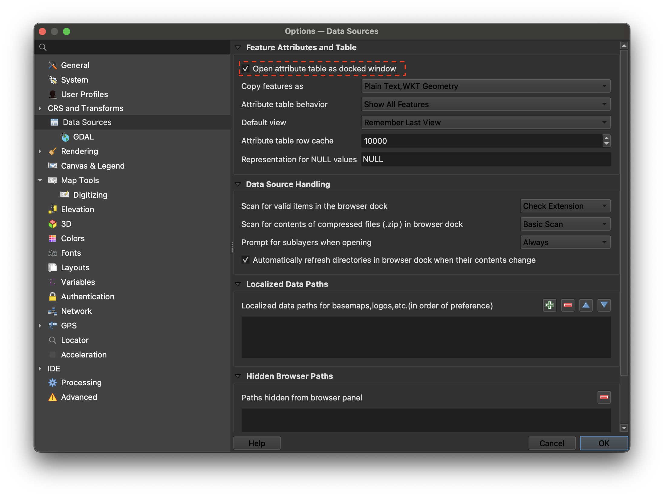
Open attribute table as docked windowYou can also toggle this setting using the right-most button at the top of the attribute table.
Throughout this section, you’ll write expressions to query and calculate data. The syntax matters:
- Double quotes reference column names:
"street_name","population" - Single quotes denote text values:
'residential','Madrid' - No quotes for numbers and built-in functions:
100,mean(),$length $prefix indicates built-in geometry properties:$length,$area,$perimeter
Example: "division_desc" = 'food_bev' finds rows where the division_desc column equals the text value food_bev.
Getting this wrong is a common source of errors. "food_bev" looks for a column named food_bev. 'food_bev' is a literal text value.
Modifying data
The attribute table in QGIS allows you to modify existing data and add new columns to store additional information.
- Toggle Editing Mode by clicking the Toggle Editing Mode button (pencil icon).
In this mode, you can edit the contents directly, for example, you can edit the street names if you wish. In this case, let’s instead add a new field called length and we’ll assign the street lengths to this new attribute:
- Click on the
New Fieldbutton in the toolbar - Set the Name as
lengthand the type asDecimal number, thenOK. - Check that the “Only update selected” option is not selected.
- Open the Field Calculator by clicking its icon (abacus symbol) in the toolbar.
- Select
Update existing fieldand select thelengthcolumn. - In the
Expressionpane, enter$length, then press the blue forward button below to preview the results. This expression extracts the length of each LineString geometry. - Press
OKand check that your length column has been updated. The above expression will have been applied to each row individually, saving the measured length of the LineString geometries into the newlengthcolumn. - Press the
Save editsbutton to save your calculation. - Turn off editing mode.
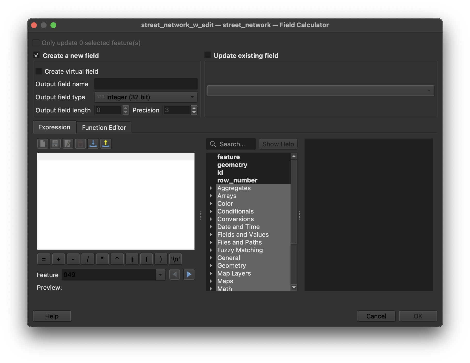
The field calculator is a window that you will keep coming back to over and over again. Take some time to understand the following parts:
Only update X selected feature(s)Create a new field/Update existing field- Expression box
- Function list / helper
- Preview
Remember to navigate this window from left to right, top to bottom. Certain fields will only be enabled according to previous choices.
Selecting and Filtering
Expressions let you query your data using attribute values. Instead of manually scrolling through thousands of rows, you can select exactly what you need. Let’s filter the premises data by landuse types.
- Open the premises data Attribute Table.
- Explore the landuse types, pay attention to the
division_descandepigraph_desccolumns. For this case, we’ll select all features with adivision_descvalue offood_bev. - Open the
Select features using expressionpanel (yellow icon with Epsilon symbol). - Type in
"division_desc" = 'food_bev'– here we are referencing the column name and we’re filtering all rows where column values equal the string value of'food_bev'. Notice the use of double quotes for column names and single quotes to denote a string. - Click
Select Features– you should now see all relevant rows highlighted. - Export the premises to a new GeoPackage called
prems_food_bev.gpkg, making sure thatSave only selected featuresis selected.
You now have a separate layer containing only food and beverage locations. Remove the original madrid_premises layer from the map.
Manipulating Columns
There is a sneaky issue in the file, which we’ll fix: The epigraph_desc column name actually contains a trailing space after the visible text characters. This will cause confusion because it will trigger errors when used in expressions by someone possibly unaware of the space in the column name: QGIS expressions won’t be able to find the column if typed without the trailing space.
Let’s create a new column name without spaces. We’ll create a copy of the original data and we’ll then delete the original column:
- Open the Attribute Table and enter edit mode.
- Click the
Open field calculatorbutton. - Select
Create a new field - Use
epigraph_desc_fixfor the name andText (string)for the type. - Use
"epigraph_desc "for the expression. Notice the double quotes (denoting a column name) and the intentional trailing space. Without that space, QGIS would look for a column calledepigraph_descwhich doesn’t exist. - This expression tells QGIS to simply reuse the values from the existing
"epigraph_desc "column without further modification. - Click
OK.
You’ll now see a new column called epigraph_desc_fix added to your Attribute Table, with values matching the original. We can now delete the original column:
- Click the
Delete fieldbutton. - Select the column with the trailing space (it will appear as
epigraph_descfollowed by a space) and clickOK. - Toggle editing mode and save.
Filtering Map Views
Expressions are also useful for filtering the visibility of features in the map view. For example, using the new prems_food_bev layer:
- Right click the layer in the Layer Panel and select
Filter... - Type an expression using the columns and available functions, for example:
"epigraph_desc_fix" = 'BAR RESTAURANTE' - Click to
TestorClearyour expressions.
If all you want is to work with a subset of the data without creating a separate file you can use the Filter... option. However, if editing, remember that the entire file is still stored locally and you are only seeing/editing a subset.
Lab Work
Challenge: Deleting Features
Select all features where epigraph_desc_fix has a value of BAR CON COCINA and delete them. Note that there is a Delete selected features button in the toolbar.
Deleting features is permanent once you save. If you make a mistake, toggle off editing mode without saving to discard changes.
- Open the Attribute Table and enter edit mode.
- Select by expression using
"epigraph_desc_fix" = 'BAR CON COCINA', and close the panel - Click
Delete selected features(trash can icon). - Toggle editing mode and save.
Challenge: Select and Export
From the prems_food_bev layer, select all CAFETERIA features and save to a separate new GeoPackage called prems_cafeteria.
- Open the Attribute Table.
- Select by expression using
"epigraph_desc_fix" = 'CAFETERIA', and close the panel. - Export the premises to a new GeoPackage called
prems_cafeteria.gpkg, making sure thatSave only selected featuresis selected.
Challenge: Categorising Street Lengths
Switch to the street_network layer. Add a street_cat column to classify streets by length. Set the value to long where the street is greater than average length for Madrid, and short otherwise.
- Your expression will need to use a greater-than
>symbol and a built-inmean()function (“mean” is the statistical term for “average”). - Note the
Toggle multi edit modebutton which enables edits of all selected features at once. - Note the
Invert selectionbutton.
- Open the Attribute Table and toggle edit mode.
- Click on the
New Fieldbutton in the toolbar - Set the Name as
street_catand the type asText (string), thenOK. - Select by expression using
$length > mean($length), and close the panel. - Click the
Toggle multi edit modebutton, typelongin thestreet_catfield and apply changes. This will update thestreet_catcolumn for all currently selected features. - Click the
Invert selectionbutton, typeshortin thestreet_catfield and apply changes. - Toggle multi edit and edit modes and save changes.
Alternatively, there are more advanced expression options involving if-else logic. In this case, the Field Calculator can be used to update the fields directly:
- Open the Field Calculator by clicking its icon (abacus symbol) in the toolbar.
- Select
Create a new fieldand set the Name asstreet_catand the type asText (string). This assumes you’ve not already created the column. - Use the expression
if ($length > mean($length), 'long', 'short'). This will set the value tolongif greater than average length, elseshort.
Note that you can search for functions such as if() or mean() in the searchbox (in the Field Calculator) and that clicking on the relevant result shows documentation explaining how the function can be used, along with some examples.
Challenge: Create (and Save) a Style
Using the newly created street_cat column, visualize the streets with a categorical color set. Save this style under the name Above/below avg length.
- Open the Layer Styling panel (View → Panels → Layer Styling)
- Change the style type from Single Symbol to Categorized
- Set the Value dropdown to
street_cat - Click Classify to generate categories for
longandshort - Adjust colours as desired
- Right-click the layer → Styles → Rename Current
- Enter
Above/below avg length
Bonus Advanced Challenge
For more than two categories, you’ll need a CASE expression. This works like a series of if-then checks:
CASE
    WHEN condition1 THEN 'result1'
    WHEN condition2 THEN 'result2'
    ELSE 'default'
END
QGIS evaluates conditions in order and uses the first match.
Add a new street length category called street_5cats and prepare an associated style based on the following 5 categories:
shortest(less than 50% of the average length)shortabout average(within +- 5% of the average length)longlongest(greater than 150% of the average length)
If you already know some statistics, you can adapt the above categorisation to use quartiles (q1, median, q3) or standard deviations (stdev) instead of percentage thresholds.
- Open the Field calculator
- Create a new field
street_5catsof typeText (string) - Use the expression:
CASE
    WHEN $length < 0.5 * mean($length) THEN 'shortest'
    WHEN $length < 0.95 * mean($length) THEN 'short'
    WHEN $length <= 1.05 * mean($length) THEN 'about average'
    WHEN $length <= 1.5 * mean($length) THEN 'long'
    ELSE 'longest'
END
Since CASE evaluates in order and stops at the first match, you don’t need to repeat the lower bounds. If a street reaches line 2, it’s already ≥ 0.5 × mean (otherwise line 1 would have matched).
- Add a new style named
5 categories. - Use a divergent colour range (eg.
Spectral) to denote your categorical distribution.